MIT 14.01 Principles of Microeconomics | Fall 2023 | Prof. Jonathan Gruber
Lecture 7: Competition I
한국어Core Message
"In producer theory, you're not given a budget constraint. You get to choose how much to produce. And to get that, we're going to add a third element to the model: market structure."
This lecture introduces market structure as the missing piece that determines how much firms produce. We focus on perfect competition, derive the profit maximization condition P = MC, and show how firm supply curves aggregate into market supply curves.
1. Market Structure: The Missing Piece
1.1 The Producer Theory Gap
"The one place producer theory is harder than consumer theory is you're not given a budget constraint. You get to choose how much you have. You get to choose how much to produce."
| Consumer Theory | Producer Theory |
|---|---|
| Budget given (income) | No budget constraint! |
| 2 equations, 2 unknowns | Need a 3rd element |
| Maximize utility given constraint | Must choose how much to produce |
1.2 The Three Market Structures
| Structure | # of Firms | Example | When Covered |
|---|---|---|---|
| Perfect Competition | Many (infinite) | Commodities, eBay | Now (Lec 7-8) |
| Monopoly | One | Utilities, patents | After midterm |
| Oligopoly | Few | Auto industry | After midterm |
"Oligopoly is really the way markets almost all look, which is a number of firms competing, but not too many. Think of the auto industry. There's more than one car company, but there aren't 1,000 car companies."
2. Perfect Competition: Definition and Assumptions
2.1 The Key Definition
Price-Takers: In a perfectly competitive market, all firms are price-takers. No action by any individual firm can affect the market price.
2.2 When Does This Hold? Perfectly Elastic Firm Demand
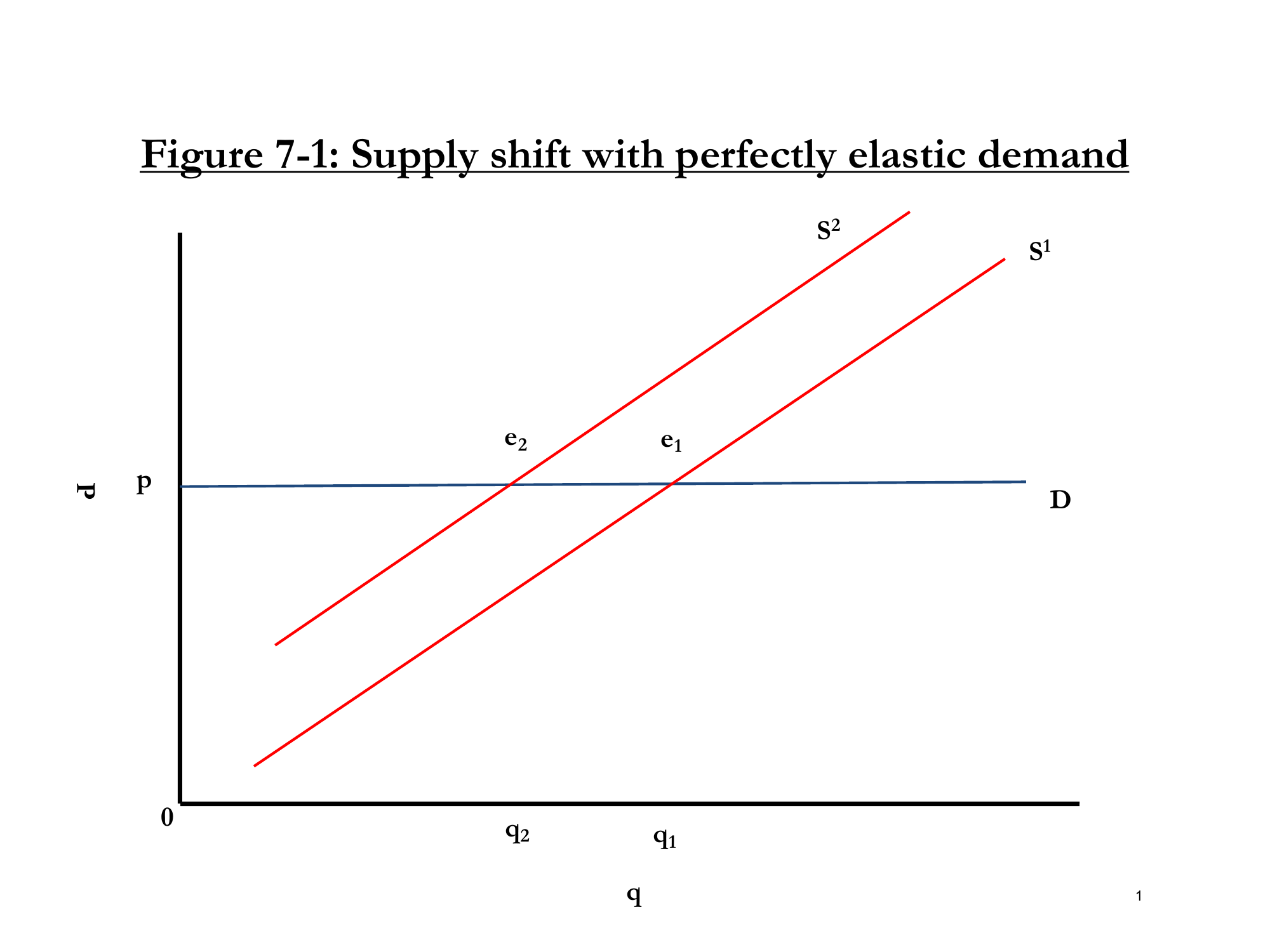
Figure 7-1: In perfect competition, each firm faces perfectly elastic demand. Note: x-axis is little q (firm), not big Q (market).
"This does not say the market demand is perfectly elastic. The demand for any given firm is very elastic. I'm not saying the demand for Eiffel Tower statuettes in general is perfectly elastic. I'm saying that across sellers, the firm-specific demand is perfectly elastic."
2.3 Three Key Assumptions
| # | Assumption | Meaning |
|---|---|---|
| 1 | Identical Products | All firms sell the exact same thing |
| 2 | Full Price Knowledge | Every consumer knows every firm's price |
| 3 | No Transaction Costs | You can easily shop at any firm |
2.4 Real-World Examples
eBay (Almost Perfect):
- Products are (somewhat) identical
- Prices are listed
- Easy to shop
But violations exist:
- Shipping costs hidden (shrouded attribute)
- Products not truly identical
- Time to search = transaction cost
The Eiffel Tower Keychain Example:
"Think of the Eiffel Tower. There are literally hundreds of guys who have spread out blankets selling the same damn little Eiffel Tower keychain. I can easily see what people are charging. They're right next to each other. There's little transaction costs. I can see it's the same damn keychain."
Result: A student verified that all sellers right near the Eiffel Tower charged identical prices! But once you got further away, prices differed (different location = not identical anymore).
3. Profit Maximization in Perfect Competition
3.1 The Firm's Objective
max π(q) = R(q) - C(q)
where R(q) = revenue, C(q) = cost
3.2 The First-Order Condition
Take derivative and set to zero:
dπ/dq = dR/dq - dC/dq = 0
MR = MC
General Rule: Marginal Revenue = Marginal Cost
3.3 In Perfect Competition: MR = P
"In a competitive market, we know what the marginal revenue is. What do you get from selling the next unit? Well, you get the market price, p. It's given to you. The marginal revenue is always p."
P = MC
The profit maximization rule in perfect competition
4. Worked Example: Finding Optimal Output and Profits
4.1 Setup
- Cost function: C(q) = 10 + 5q²
- Market price: p = 30
- Marginal cost: MC = dC/dq = 10q
4.2 Finding Optimal Quantity
Set P = MC:
30 = 10q
q* = 3
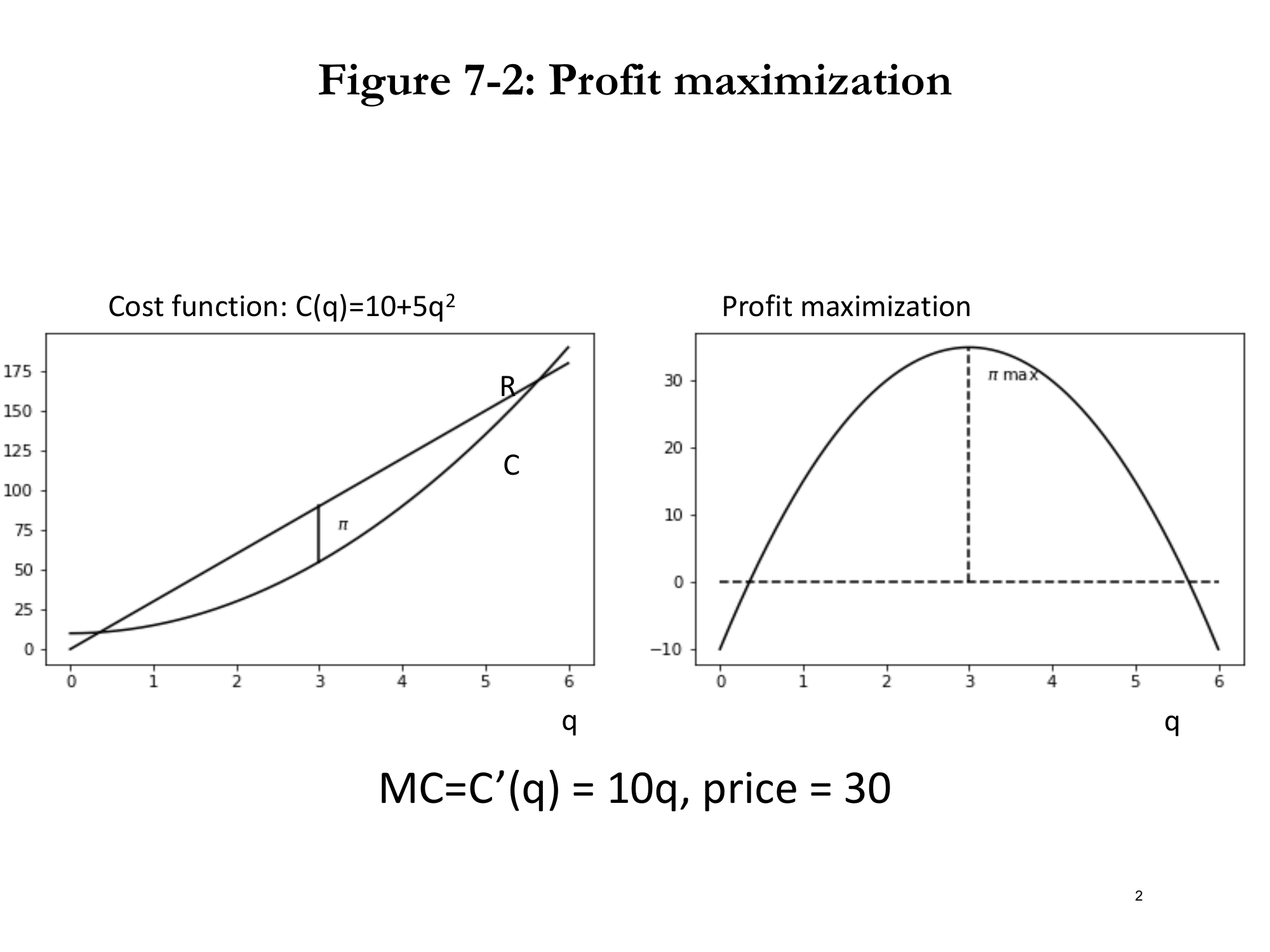
Figure 7-2: Left: Revenue (R) and Cost (C) curves. Right: Profit curve showing maximum at q = 3.
4.3 The Hill-Climbing Intuition
"Think of yourself as climbing a mountain that's in the clouds. And you're trying to get to the top of the mountain, but you can't see more than one step in front of you. If you take a step forward and you go up, you know you're heading up the mountain. Take a step forward and you go down, you're heading down the mountain."
Marginal Decision-Making:
- At q = 1, 2, 3: MR > MC → each unit adds to profit → keep going up!
- At q = 4, 5, 6: MR < MC → each unit reduces profit → going down!
- At q = 3: MR = MC → at the top of the hill
4.4 Calculating Profits
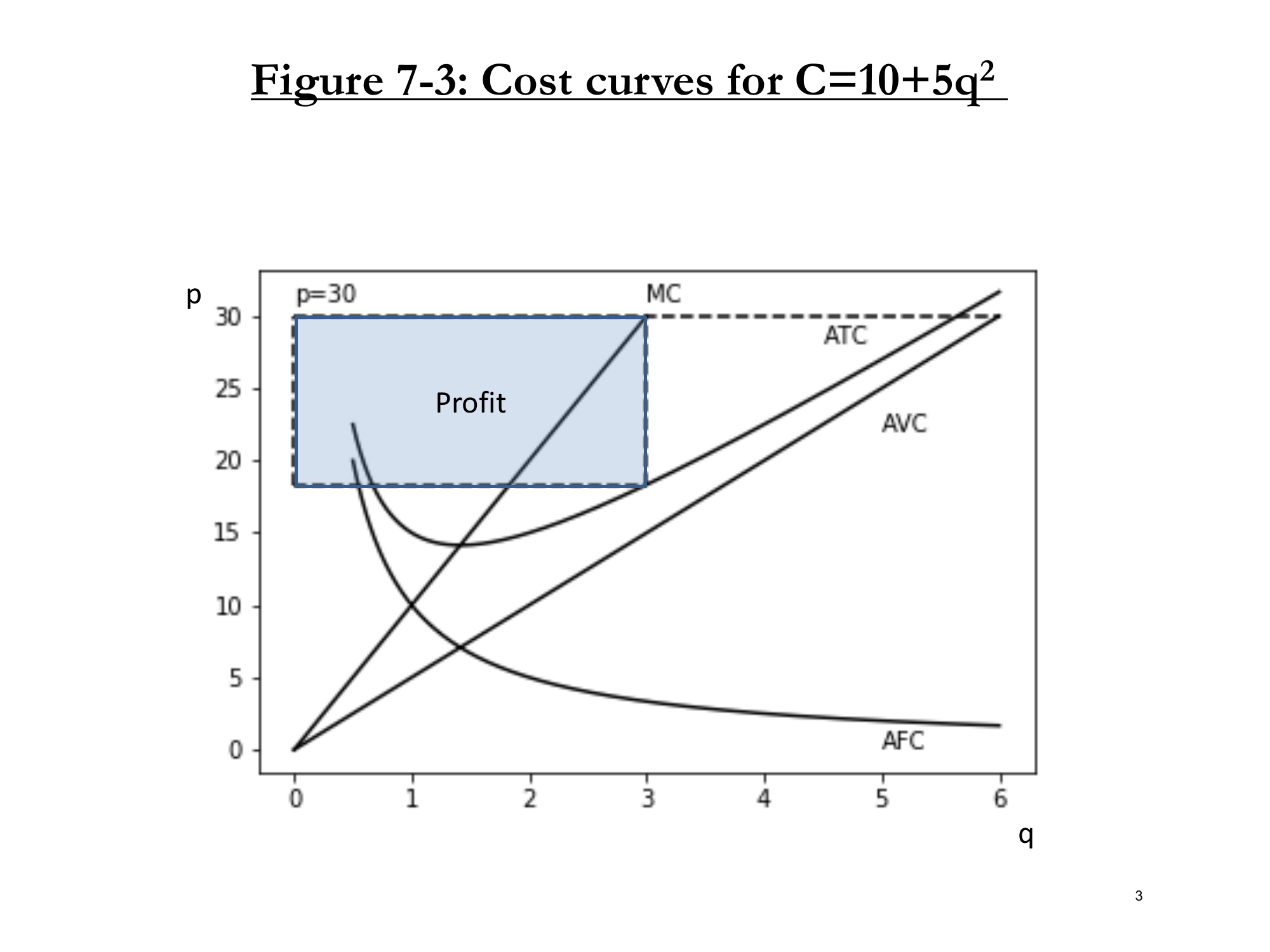
Figure 7-3: Profit = (P - ATC) × q = blue rectangle.
Step 1: Find Average Cost at q = 3
AC = C(q)/q = (10 + 5q²)/q = 10/q + 5q
AC(3) = 10/3 + 5(3) = 3.33 + 15 = 18.33
Step 2: Calculate Profit per Unit
Profit per unit = P - AC = 30 - 18.33 = 11.67
Step 3: Calculate Total Profit
π = (P - AC) × q = 11.67 × 3 ≈ 35
Profit = (Price - Average Cost) × Quantity
This is the area of the blue rectangle in Figure 7-3
5. Stress Test: What Happens with a Tax?
5.1 Adding a $10/unit Tax
Question: What happens if the firm must pay $10 per unit sold?
New cost function:
C(q) = 10 + 5q² + 10q
Note: NOT 20 + 5q². The tax is per unit, not a flat amount!
5.2 New Optimal Quantity
New MC: d(10 + 5q² + 10q)/dq = 10q + 10
Set P = MC:
30 = 10q + 10
q* = 2 (down from 3)
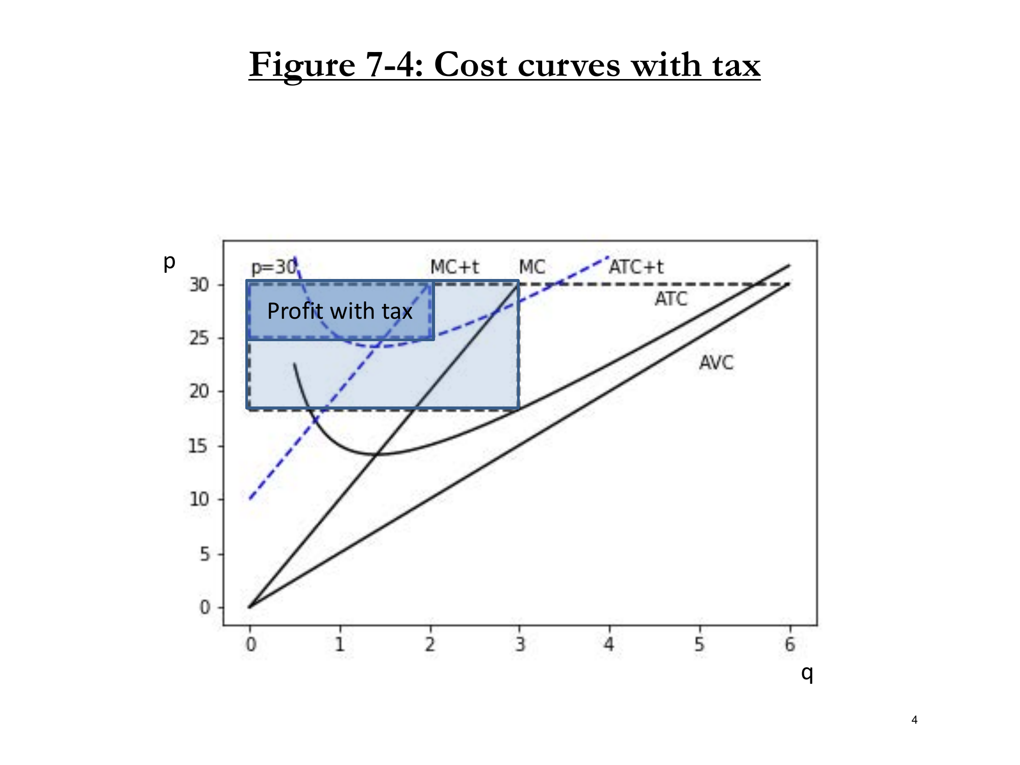
Figure 7-4: With tax, MC shifts up. Profit rectangle shrinks in both width (fewer units) and height (lower profit per unit).
5.3 Two Effects on Profits
| Effect | Before Tax | After Tax |
|---|---|---|
| Quantity (width) | 3 | 2 ↓ |
| Profit per unit (height) | 11.67 | Lower ↓ |
| Total Profit | ~35 | Much smaller |
6. The Shutdown Rule: When to Stop Producing
6.1 Key Insight: Losing Money ≠ Shutdown
"In the short run, losing money is not necessarily a reason to shut down. You can lose money and want to stay in business."
6.2 Example: Price Falls to $10
With C(q) = 10 + 5q² and p = 10:
- MC = 10q, so at p = MC: q* = 1
- Revenue = 10 × 1 = 10
- Cost = 10 + 5(1)² = 15
- Profit = 10 - 15 = -5 (losing money!)
6.3 Should You Shut Down?
If you produce q = 1: Profit = -5
If you produce q = 0: Profit = -10 (still pay fixed costs!)
Better to produce and lose 5 than shut down and lose 10!
6.4 The Shutdown Rule
Shut down when: P < AVC
Keep producing as long as price covers variable costs
"Fixed costs are, in the short run, sunk. They're irrelevant. You already paid them. You just want to ask for the next unit: Will I make money?"
6.5 In Our Example: Never Shut Down
For C(q) = 10 + 5q²:
- VC = 5q²
- AVC = 5q
- At optimum (MC = P): 10q = P → q = P/10
- So AVC = 5(P/10) = 0.5P
Since AVC = 0.5P < P always, the firm never shuts down with this cost function.
7. Deriving the Supply Curve
7.1 The Firm's Supply Decision
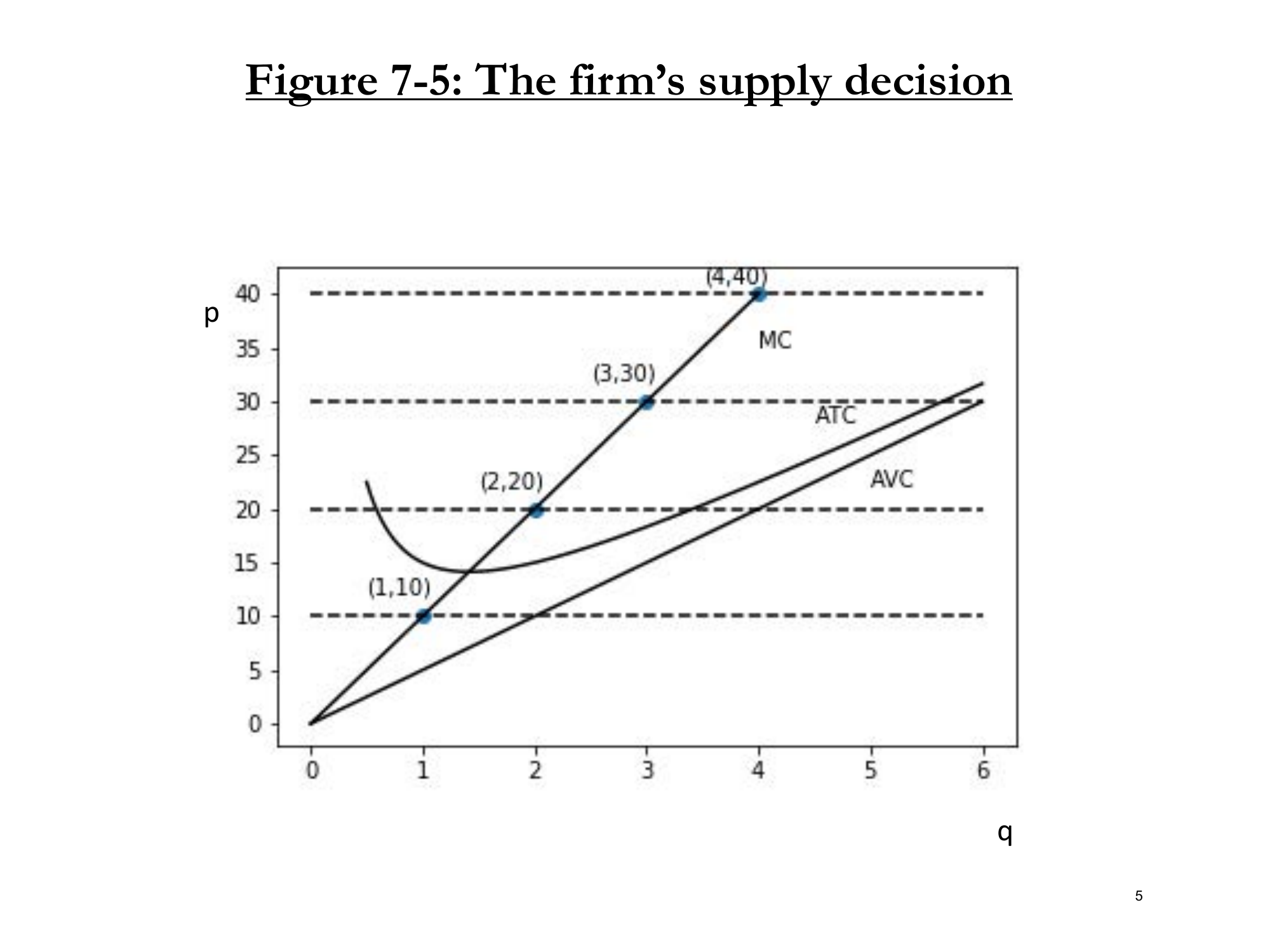
Figure 7-5: At each price, the firm produces where P = MC.
- At P = 10: produce q = 1
- At P = 20: produce q = 2
- At P = 30: produce q = 3
- At P = 40: produce q = 4
7.2 The Key Insight
The Supply Curve IS the Marginal Cost Curve
"The demand curve was the marginal willingness to pay for a good. The supply curve is the marginal cost of producing the next good."
7.3 The Short-Run Firm Supply Curve
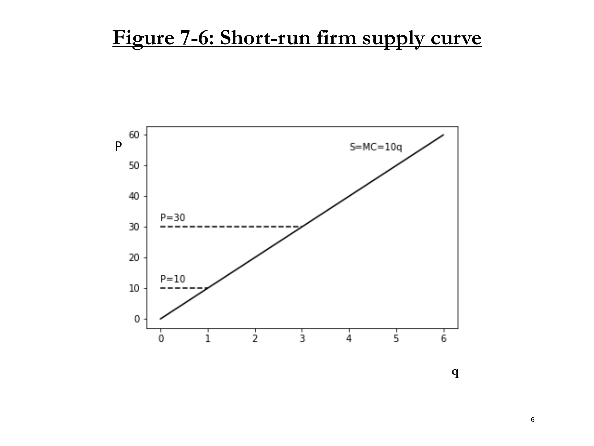
Figure 7-6: Short-run firm supply curve S = MC = 10q.
Technical Definition:
Short-run supply curve = MC curve above the shutdown point
(above minimum AVC)
7.4 Long-Run vs. Short-Run Supply
| Short Run | Long Run | |
|---|---|---|
| Supply Curve | MC above min AVC | MC (full stop) |
| Shutdown Rule | P < AVC | π < 0 |
| Why? | Can re-optimize K later | Already optimized everything |
"In the long run, if you've done all your optimizing and you're still losing money, you're just shit out of luck. You should get out of the business because there's no more optimization you can do."
8. From Firm Supply to Market Supply
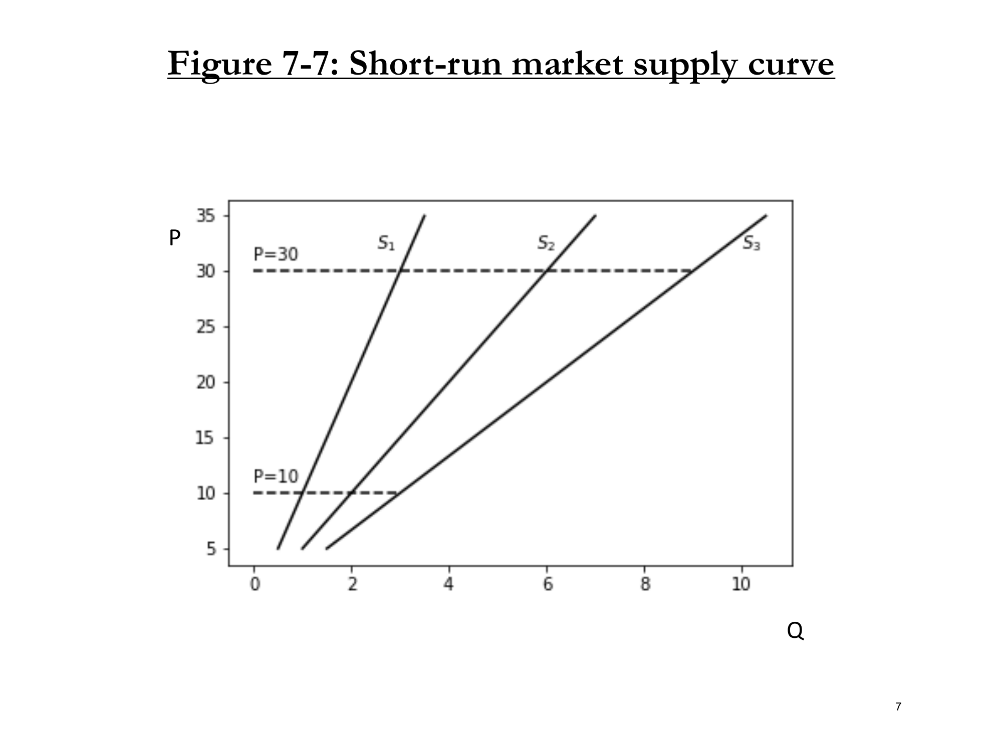
Figure 7-7: Adding identical firms makes market supply more elastic. S₁ = 1 firm, S₂ = 2 firms, S₃ = 3 firms.
8.1 Aggregating Firm Supply
With n identical firms:
- Each firm: q = P/10
- Market: Q = n × (P/10)
Example with n = 1:
- At P = 10: Q = 1
- At P = 30: Q = 3
Example with n = 2:
- At P = 10: Q = 2
- At P = 30: Q = 6
8.2 Key Insight: More Firms = More Elastic Supply
More identical firms → Flatter (more elastic) market supply curve
"If I said competitive markets have an infinite number of firms and the more firms there are, the more elastic the supply curve, think about what that implies to the supply curve..."
(We'll explore this next lecture!)
9. Putting It All Together: Full Equilibrium
"This is the beauty of being at MIT. You'll never find an introductory economics course that does this. Before Paul Samuelson taught this class, people would teach the graph and be done with it. You guys want the math? I'm giving you the math."
Step A: Get the Supply Curve
1. Start with production function: q = √(L × K)
2. Given: w = 5, r = 10, K̄ = 1
3. Derive cost function: C(q) = 10 + 5q²
4. Get MC: MC = 10q
5. Firm supply (P = MC): q = P/10
Step B: Make Market Supply Curve
Assume n = 6 firms
Q = 6 × (P/10) = 3P/5
Market supply: Q = (3/5)P
Step C: Get Demand Curve
From consumer theory: Q = 48 - P
Step D: Find Equilibrium
Set supply = demand:
(3/5)P = 48 - P
(3/5)P + P = 48
(8/5)P = 48
P* = 30
Q* = 18
Step E: Verify Individual Firm Behavior
- Market quantity Q* = 18
- With 6 identical firms: each produces q* = 18/6 = 3
- Check: At P = 30, firm sets MC = P → 10q = 30 → q = 3 ✓
The magic of the market: Everyone is satisfied!
Key Takeaways
| # | Concept | Key Point |
|---|---|---|
| 1 | Market Structure | The "third element" that determines how much to produce |
| 2 | Perfect Competition | Firms are price-takers; face perfectly elastic demand |
| 3 | Profit Max Rule | MR = MC; in competition: P = MC |
| 4 | Profit Calculation | π = (P - AC) × q = profit rectangle |
| 5 | Shutdown Rule | Short run: shut down if P < AVC; Long run: if π < 0 |
| 6 | Supply Curve | = MC curve (above shutdown point in SR) |
| 7 | Market Supply | Sum of firm supplies; more firms = more elastic |
What's Next?
Coming up: Competition II - What happens when there are infinitely many firms? Long-run equilibrium and the role of entry/exit.