MIT 14.01 Principles of Microeconomics | Fall 2023 | Prof. Jonathan Gruber
Lecture 6: Costs
한국어Core Message
"We're going to start today by talking about the key construct of producer theory, which is short-run cost curves. Remember, the way firms maximize profits is by minimizing costs, by producing goods as efficiently as possible at minimum costs."
This lecture translates production functions into cost functions, introduces the critical concepts of marginal and average costs, and shows how firms minimize costs in both the short run and long run. We also explore the crucial distinction between accounting costs and economic (opportunity) costs.
1. From Production Function to Cost Function
1.1 Why Do We Care About Costs?
"Remember, the way firms maximize profits is by minimizing costs, by producing goods as efficiently as possible at minimum costs."
Last lecture, we developed the production function. Now we translate that into costs, because that's what firms actually control.
1.2 The Cost Function
Definition: The cost function C(q) tells us the total cost of producing quantity q.
C(q) = r·K̄ + w·L(q)
where r = rental rate of capital, w = wage, K̄ = fixed capital, L(q) = labor needed for q
1.3 Deriving the Cost Function: A Worked Example
Given:
- Production function: q = √(L × K)
- Wage: w = 5
- Rental rate: r = 10
- Fixed capital: K̄ = 1
Step 1: Solve production function for L
q = √(L × K̄) → q² = L × K̄ → L = q²/K̄
Step 2: Substitute into cost function
C(q) = r·K̄ + w·L = 10(1) + 5(q²/1) = 10 + 5q²
Final Cost Function: C(q) = 10 + 5q²
"Where do w and r come from? I'll teach you that in a few lectures. Remember, we peel the onion in this class. We're revealing the mystery slowly. Right now, just take those as given."
2. Types of Costs
2.1 Key Definitions
| Cost Type | Definition | In Our Example | Formula |
|---|---|---|---|
| Fixed Costs (FC) | Costs that do NOT vary in the short run | 10 | r·K̄ |
| Variable Costs (VC) | Costs that CAN vary in the short run | 5q² | w·L(q) |
| Total Costs (TC) | Sum of fixed and variable costs | 10 + 5q² | FC + VC |
2.2 Marginal Cost: The Key Concept
Marginal Cost (MC): The cost of producing one more unit
MC = dC/dq = dVC/dq
(In short run, dTC/dq = dVC/dq because fixed costs don't change)
In our example:
MC = d(10 + 5q²)/dq = 10q
2.3 Average Costs
| Average Cost Type | Formula | In Our Example |
|---|---|---|
| Average Fixed Cost (AFC) | FC/q | 10/q |
| Average Variable Cost (AVC) | VC/q | 5q |
| Average (Total) Cost (AC) | TC/q = AFC + AVC | 10/q + 5q |
3. Cost Curves: Graphical Analysis
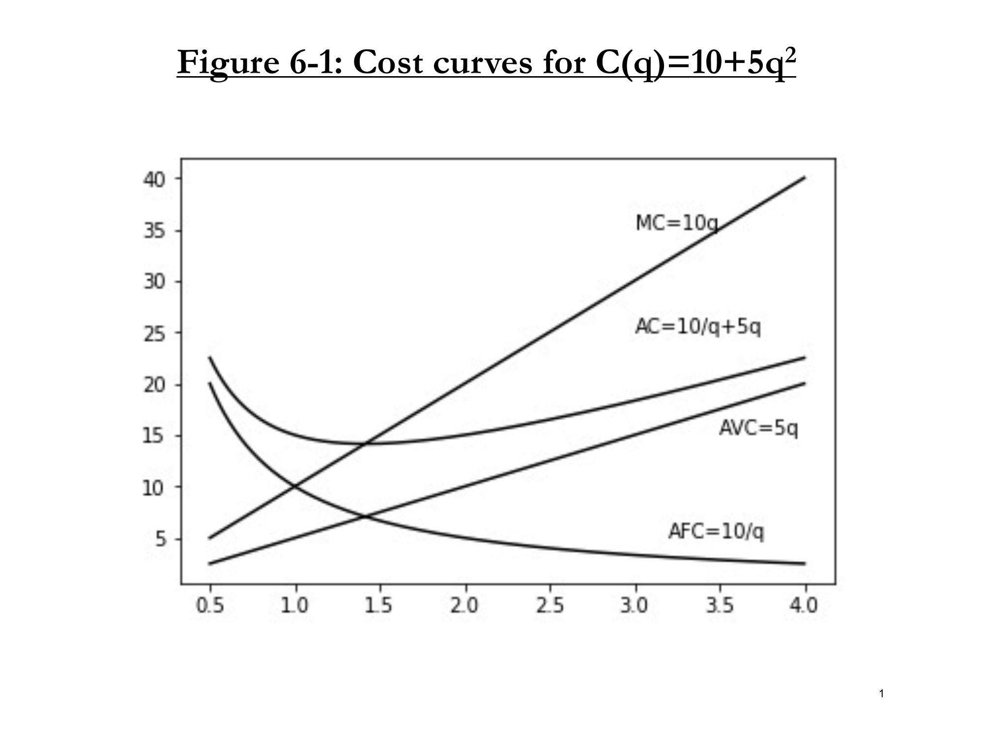
Figure 6-1: Cost curves for C(q) = 10 + 5q². Shows MC, AC, AVC, and AFC.
3.1 Understanding the Shapes
| Curve | Shape | Why? |
|---|---|---|
| MC = 10q | Upward sloping (linear) | Each additional unit costs more (diminishing returns to labor) |
| AFC = 10/q | Always falling (hyperbola) | Fixed costs spread over more units |
| AVC = 5q | Always rising (linear) | Diminishing marginal product of labor |
| AC = 10/q + 5q | U-shaped (first falls, then rises) | AFC pulls it down at first, then AVC pulls it up |
3.2 Why Average Cost is U-Shaped
"Average costs first fall, then rise. Why is that? Well, that's because at first, you have these big fixed costs you have to pay off. But over time, the fixed costs get smaller relative to the variable costs."
3.3 Critical Relationship: MC Intersects AC at Minimum
Key Rule: Marginal Cost crosses Average Cost at the minimum of Average Cost.
Intuition:
- If MC < AC: Producing one more unit brings down the average → AC is falling
- If MC > AC: Producing one more unit brings up the average → AC is rising
- At MC = AC: Average is neither rising nor falling → minimum!
"Wherever the marginal cost is above the average cost, the average cost is rising. Wherever the marginal cost is below the average cost, it's falling. Therefore, marginal cost intersects average cost at the minimum."
4. The Link Between Marginal Cost and Marginal Product
4.1 Deriving the Relationship
Starting from: C = r·K̄ + w·L
Differentiate with respect to q:
MC = dC/dq = w · (dL/dq)
But recall: MPL = dq/dL, so dL/dq = 1/MPL
MC = w / MPL
4.2 Interpretation
"The marginal cost of producing the next unit of the good is higher the more you have to pay each worker and lower the more productive each worker is."
| If... | Then MC... | Intuition |
|---|---|---|
| w ↑ (wage rises) | MC ↑ | More expensive labor → higher cost per unit |
| MPL ↑ (productivity rises) | MC ↓ | Each worker produces more → need fewer workers per unit |
| MPL ↓ (diminishing returns) | MC ↑ | This is why MC curves slope upward! |
5. Sunk Costs: A Critical Distinction
5.1 Fixed vs. Sunk Costs
"Last lecture, I said in the long run, all inputs are variable. I'm going to already contradict that. We have some costs which in the long run are not variable. Those are called sunk costs."
| Cost Type | Definition | Can You Recover It? | Example |
|---|---|---|---|
| Fixed Cost | Fixed in short run, variable in long run | Yes (sell it) | Machine, building |
| Sunk Cost | NEVER recoverable, even in long run | No (gone forever) | Med school, advertising |
"A sunk cost is something you can't ever get rid of or sell. The best example would be med school. If you want to be a doctor, you have to go to med school. Having gone to med school, you can't ever un-go to med school. You have paid that cost of time and money, and you're done. It's sunk."
5.2 The Sunk Cost Fallacy
"Sunk costs are irrelevant to decision making once they're paid."
"Or as the economists say, sunk costs are sunk. Doesn't matter. It's irrelevant."
5.3 The Journey Concert Example
Gruber's Story:
- Bought Journey concert tickets for $125 each ($250 total)
- Looked at setlist, realized he only likes 3 songs
- Decided to sell tickets on StubHub
Question: How should the $250 he paid affect the price he sets on StubHub?
Answer: It shouldn't! It's a sunk cost.
"I paid it already. It's irrelevant. It's done. I already paid the 250. It's gone. I might feel sad, but it's gone."
5.4 What SHOULD Determine the Price?
The opportunity cost of going!
- If you literally don't want to go → willing to sell for $0
- If you'd pay $50 to go → set minimum price at $50
- If someone pays more than your value → sell
- If someone pays less than your value → keep tickets and go
"The amount I should be willing to get should be determined by the opportunity cost of going, not by what I paid for them."
5.5 Student Q&A: "But I Want to Recover My Sunk Costs!"
Student: "I feel like I would think about trying to recover those sunk costs."
Gruber: "Yeah, you would because that's the way humans think. But it's wrong."
"Let me put it this way. Let's say I could go online and sell them for $500 each. Should I only sell them for $250 because that's what I paid for them? No, sell them for $500. So it's irrelevant that I paid $250."
6. Long-Run vs. Short-Run Costs
6.1 The Key Intuition
Long-run costs ≤ Short-run costs (always!)
"Long-run costs will always be at the lower bound of short-run costs. The cost of production in the long run are always the same or lower than the cost of production in the short run."
Why? "The more variables you have to toy with, the more you can optimize."
6.2 LRAC as Envelope of SRAC Curves
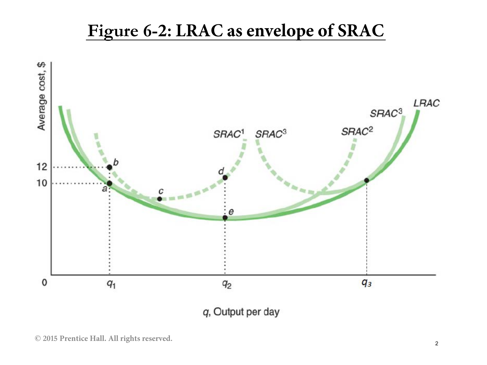
Figure 6-2: Long-Run Average Cost (LRAC) as the envelope of Short-Run Average Cost curves.
6.3 Understanding the Graph
Think of this as three different plant sizes (different K̄ choices):
- SRAC¹: Small plant (low K̄) - efficient at low output q₁
- SRAC²: Medium plant - efficient at medium output q₂
- SRAC³: Large plant (high K̄) - efficient at high output q₃
"If the firm wants to produce q₁, the most efficient K̄ is the one that yields SRAC¹. If the firm wants to produce q₃, the most efficient K̄ is the one that yields SRAC³."
6.4 Real-World Example: Tesla
The Tesla Battery Factory Story:
| Year | Situation | Plant Size |
|---|---|---|
| 2013 | Tesla founded, Musk expects to sell 20,000 cars by 2017 | Built small plant (SRAC¹) |
| 2017 | 200,000 person waiting list! Demand = q₃, not q₁ | Wrong plant size! |
| After 2017 | Built largest battery plant in world (Nevada) | Re-optimized to SRAC³ |
"Elon Musk did not produce most efficiently in the short run, so he built a bigger plant. Will he now produce most efficiently? It depends on whether demand is up at q₃ or somewhere else."
7. Cost Minimization in the Long Run
7.1 The Isocost Line
Isocost Line: All combinations of L and K that cost the same total amount.
C = w·L + r·K
Rearranging: K = C/r - (w/r)·L
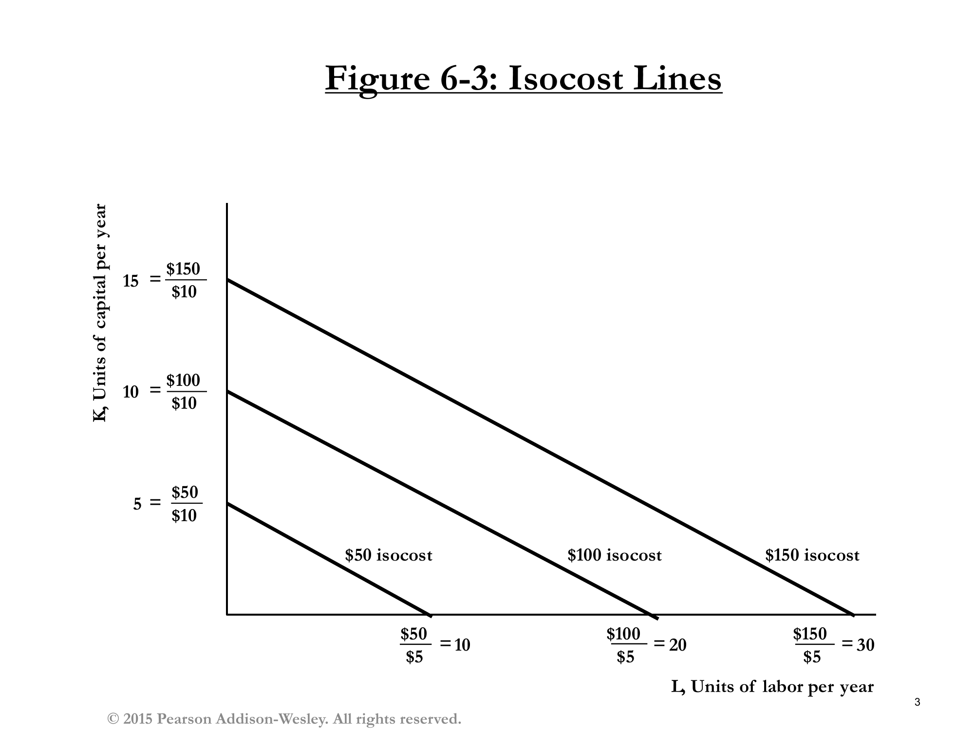
Figure 6-3: Isocost lines for w=$5, r=$10. Each line shows combinations of L and K that cost the same.
7.2 Properties of Isocost Lines
| Property | Value | Interpretation |
|---|---|---|
| Slope | -w/r = -5/10 = -1/2 | Give up 1/2 unit of K to get 1 unit of L (at same cost) |
| L-intercept | C/w | Maximum L if spend all on labor |
| K-intercept | C/r | Maximum K if spend all on capital |
7.3 The Cost Minimization Problem
Goal: For any given output q, find the combination of L and K that minimizes cost.
Solution: Find the tangency between the isoquant (from production function) and the isocost line.
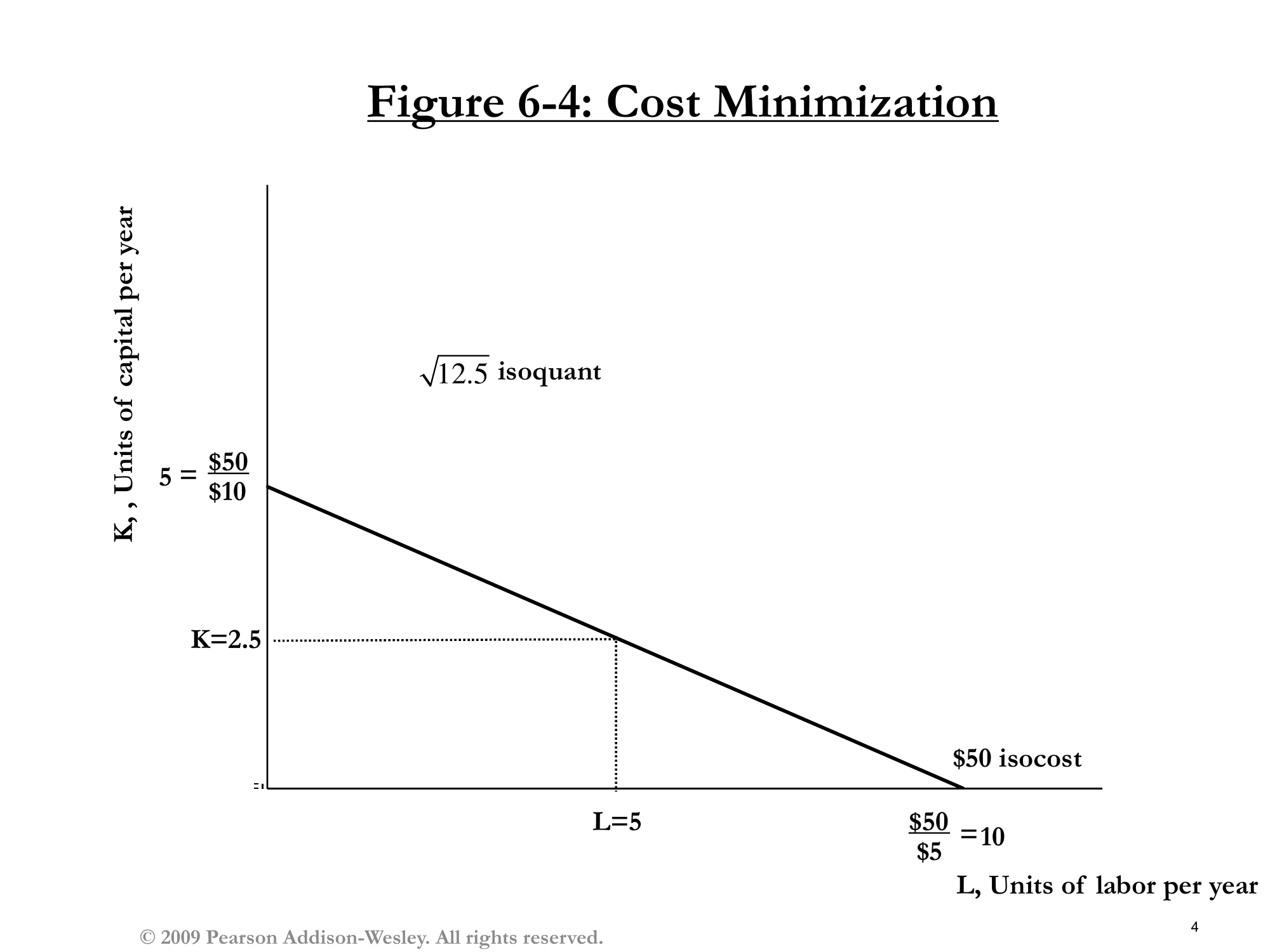
Figure 6-4: Cost minimization at tangency. To produce √12.5 units at minimum cost ($50), use L=5 and K=2.5.
7.4 The Tangency Condition
At the optimum:
Slope of Isoquant = Slope of Isocost
MRTS = -MPL/MPK = -w/r
7.5 Why Producer Theory is Harder than Consumer Theory
"This is why producer theory is harder. Because I didn't tell you the right isocost. With consumer theory, I gave you a budget constraint. I'm not giving you an isocost here. I'm just saying there are multiple possible isocosts."
| Consumer Theory | Producer Theory |
|---|---|
| Budget is fixed (given income) | Budget is a choice (how big to be) |
| 2 equations, 2 unknowns → solution | 2 equations, 2 unknowns → formula only |
| Done at tangency! | Need to choose q first! |
8. The Long-Run Expansion Path
8.1 Definition
Long-Run Expansion Path: The set of cost-minimizing combinations of L and K for every possible output level q.
8.2 Linear Expansion Path
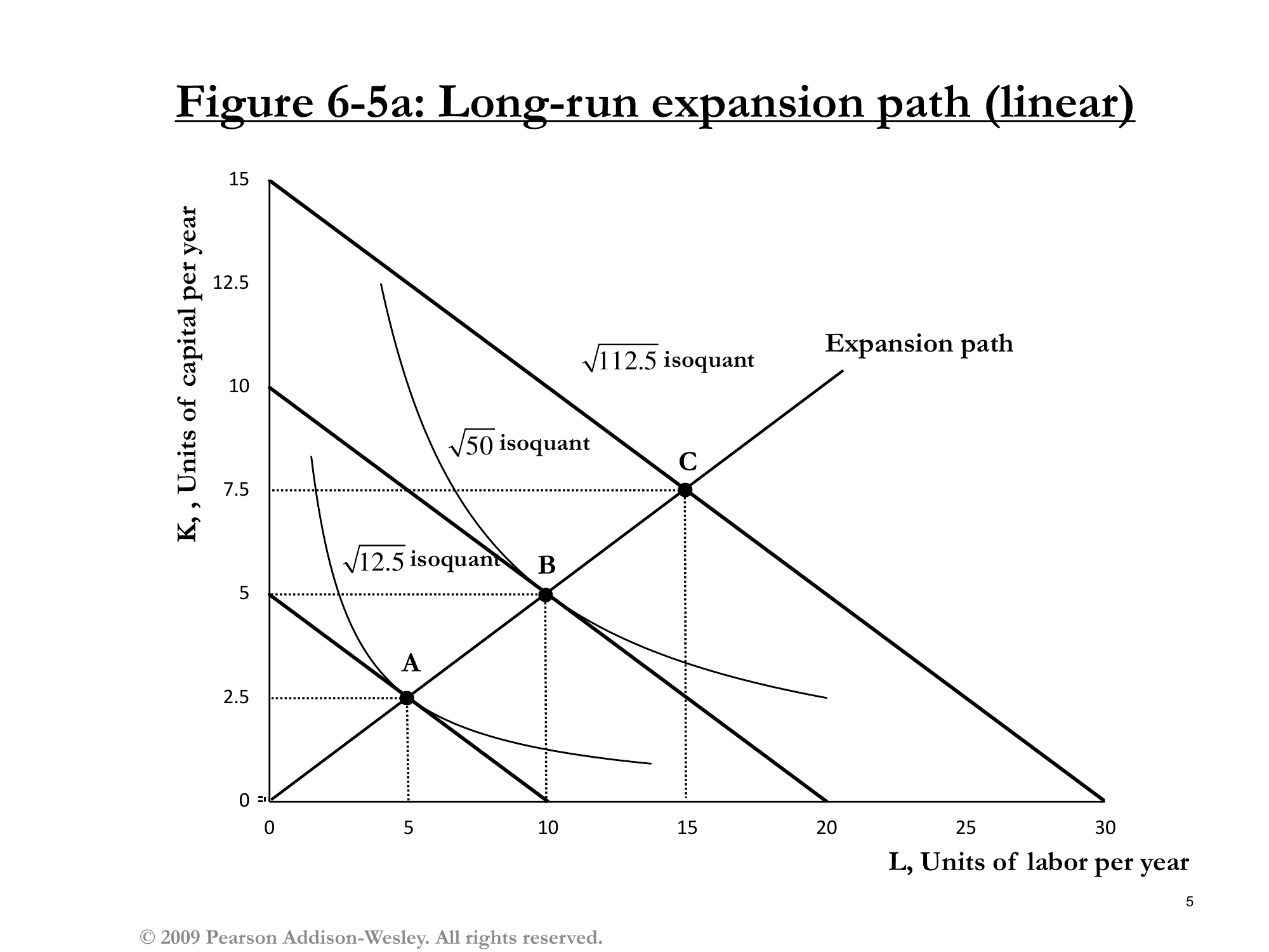
Figure 6-5a: Linear expansion path for q = √(L×K). Always use K = L/2.
8.3 Non-Linear Expansion Paths
The expansion path doesn't have to be linear. It depends on the production function.
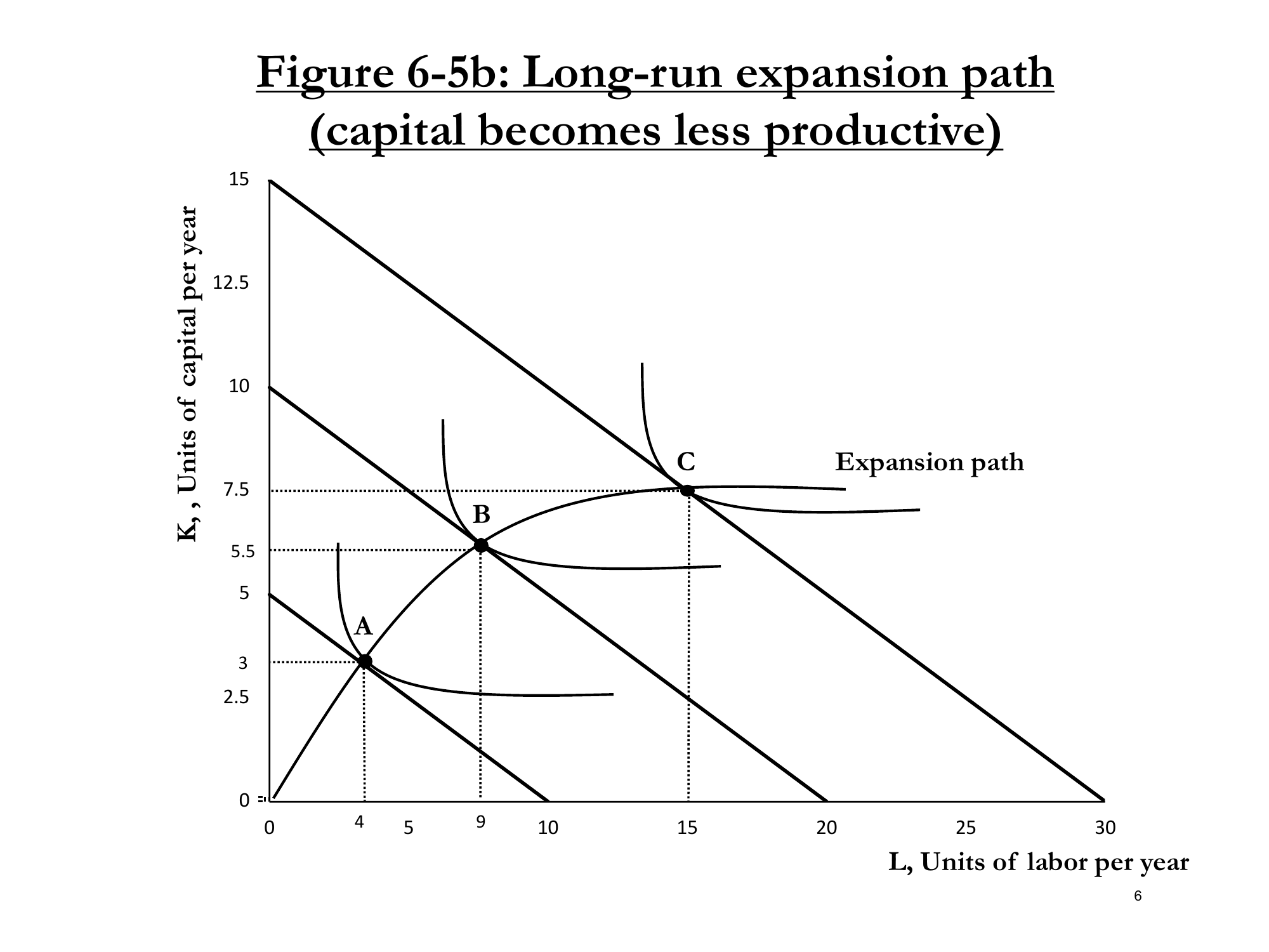
Figure 6-5b: Capital becomes less productive
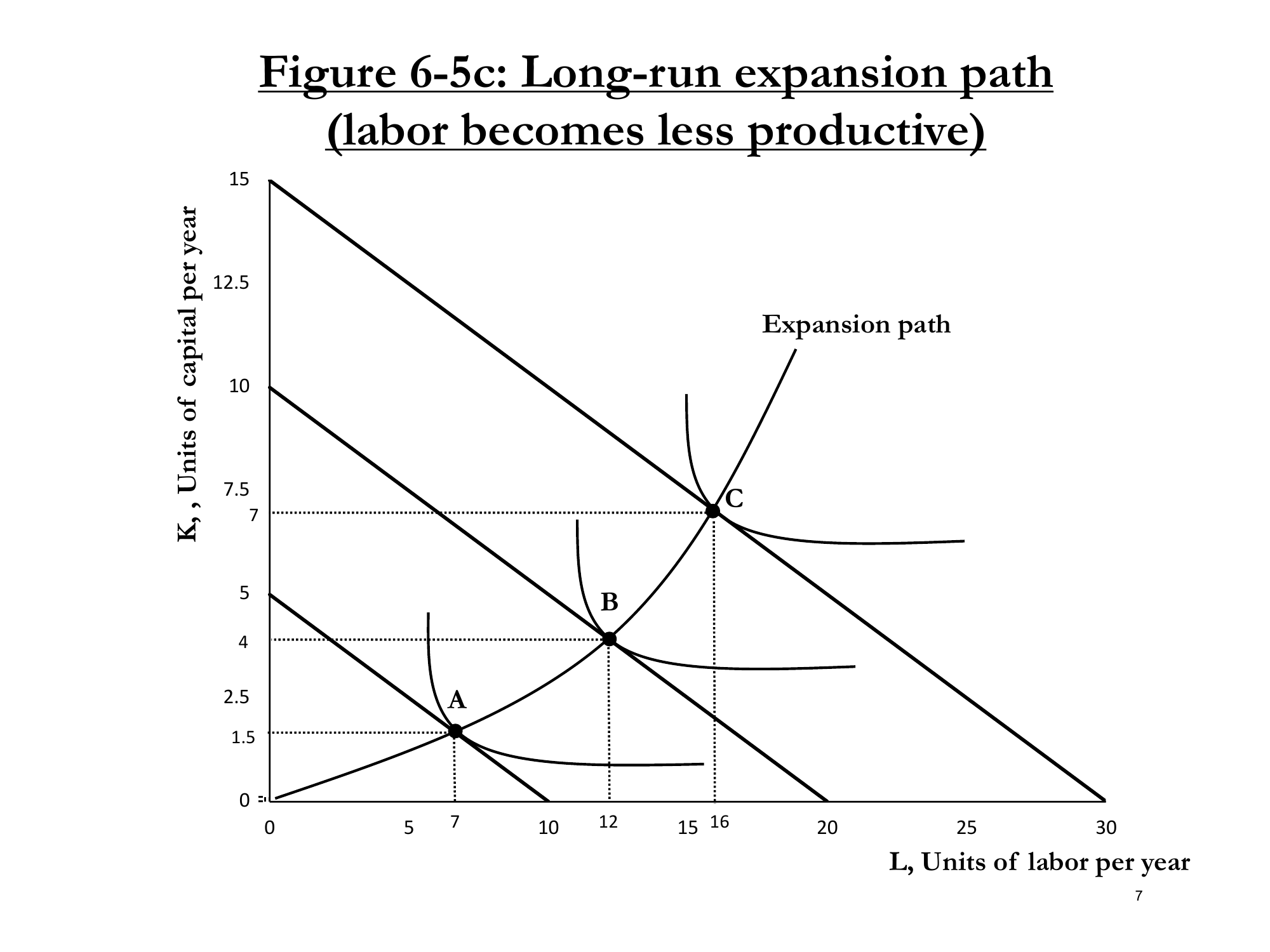
Figure 6-5c: Labor becomes less productive
8.4 Comparing the Expansion Paths
| Figure | Pattern | Real-World Example |
|---|---|---|
| 6-5a (Linear) | K/L stays constant | Standard Cobb-Douglas |
| 6-5b | L increases faster than K | "McDonald's - once you have the fry-o-later, what matters is more workers" |
| 6-5c | K increases faster than L | "Heavy machinery plant - want more machines, fewer workers" |
9. Measuring Costs: Accounting vs. Economics
9.1 The Key Difference
"This is where I get to tell you that economics is just cooler than accounting. And let me explain why. Accounting only considers the cash-flow costs that you have when you start a firm. Economics more appropriately considers opportunity costs, as well."
| Type | Definition | Includes |
|---|---|---|
| Accounting Costs | What you actually spend (cash outflows) | Wages, rent, materials, etc. |
| Economic Costs | Opportunity costs of ALL resources | Accounting costs + foregone alternatives |
9.2 The Web Design Startup Example
Scenario: You (MIT graduate) start a web design firm after graduation.
- You work full time (no salary to yourself)
- Hire one programmer for $40,000/year
- Give programmer your extra computer (1 year left before it's useless)
- After 1 year, revenue = $60,000
9.3 Two Different Perspectives
| Accounting Mom 👩💼 | Economics Dad 👨🏫 | |
|---|---|---|
| Revenue | $60,000 | $60,000 |
| Programmer salary | -$40,000 | -$40,000 |
| Your foregone salary | $0 (not counted) | -$100,000 |
| Computer (could have sold) | $0 (not counted) | -$1,000 |
| Total Costs | $40,000 | $141,000 |
| Profit | +$20,000 😊 | -$81,000 😱 |
9.4 The Lesson
"Opportunity costs are real costs. Opportunity costs are the value of the next best foregone alternative."
"Remember, that's why we call economics the dismal science. We point out nothing is free. Your time wasn't free. The time you dedicate to this firm meant you could have been doing something else. And that's not free."
Key Takeaways
| # | Concept | Key Point |
|---|---|---|
| 1 | Cost Function | C(q) = FC + VC; derived from production function |
| 2 | Marginal Cost | MC = dC/dq = w/MPL; rises due to diminishing returns |
| 3 | Average Cost | U-shaped; MC crosses AC at minimum |
| 4 | Sunk Costs | Irrelevant to decisions once paid ("sunk costs are sunk") |
| 5 | LRAC ≤ SRAC | More variables to optimize = lower costs possible |
| 6 | Cost Minimization | Set MRTS = w/r (tangency of isoquant and isocost) |
| 7 | Expansion Path | Cost-minimizing L,K combinations for all output levels |
| 8 | Opportunity Costs | Economic costs include foregone alternatives (accounting ≠ economics) |
What's Next?
"Next lecture, I will introduce the one extra step that lets you choose q."
Coming up: How firms decide how much to produce (choosing q) → Supply curve derivation