MIT 14.01 Principles of Microeconomics | Fall 2023 | Prof. Jonathan Gruber
Lecture 5: Production Theory
한국어Core Message
"Today, we are going to turn from the consumer side of the story to the producer side of the story. Once again, in the first lecture, we talked about supply and demand curves. The last few lectures, we developed where demand curves come from. Now we'll develop where supply curves come from."
This lecture marks a major transition in the course. Just as consumers maximize utility, firms maximize profits. Since demand and competition are largely outside the firm's control, maximizing profits essentially means minimizing costs. The mathematics of producer theory will closely parallel consumer theory—this is intentional and makes the material easier to learn.
Course Progress
| Lec 1 | Supply & Demand Introduction | ✓ Done |
| Lec 2-4 | Consumer Theory → Demand Curves | ✓ Done |
| Lec 5+ | Producer Theory → Supply Curves | ← Starting |
1. What Do Firms Want?
1.1 The Parallel Between Consumers and Firms
Just as we asked "What do consumers want?" (maximize utility given budget constraint), we now ask "What do firms want?"
| Agent | Goal | Subject to | Tools |
|---|---|---|---|
| Consumer | Maximize Utility | Budget Constraint | Indifference Curves, MRS |
| Firm | Maximize Profits | Production Technology | Isoquants, MRTS |
1.2 What Determines Firm Profits?
Profits (π) = Revenue - Costs = P × Q - C(Q)
Profits depend on three things:
| Factor | Firm Control? | Notes |
|---|---|---|
| 1. Consumer Demand | Limited | Advertising can affect demand, but largely given by market conditions |
| 2. Competition | Limited | Monopolies can affect market structure, but in standard competitive model, taken as given |
| 3. Costs of Production | Yes! | This is what the firm controls—how efficiently it produces |
Key Insight: "From the firm's perspective, maximizing profits is the same as minimizing costs. The way to maximize profits is to minimize costs. And that's how the firm produces as efficiently as possible, by minimizing costs."
1.3 Why Focus on Cost Minimization?
Mathematical Intuition:
π = P × Q - C(Q)
If P and Q are determined by market forces (demand and competition), then:
max π ⟺ min C(Q) for any given Q
In the real world, there are complications, but in our model—and in most of the real world—we say firms' goal is to minimize costs.
2. Production Functions
2.1 The Firm as a Black Box
To understand how to minimize costs, we need to understand where a firm's costs come from. To understand that, we need to understand what firms actually do.
Inputs
Labor (L)
Capital (K)
Labor (L)
Capital (K)
→
Production Function
q = f(L, K)
q = f(L, K)
→
Output
Goods & Services (q)
Goods & Services (q)
"In this course, firms are simply black boxes for much of the course. They're simply boxes where inputs go in and outputs come out. And in the middle is something called a production function. That production function is the magic that makes—is the magic of the firm."
2.2 Formal Definition
Production Function: A mathematical description of what is technically feasible for the firm to produce given its inputs.
q = f(L, K)
where q = output, L = labor, K = capital
2.3 Comparing Utility and Production Functions
| Aspect | Utility Function | Production Function |
|---|---|---|
| What it represents | How goods → happiness | How inputs → output |
| Tangibility | Abstract (can't measure happiness) | Concrete (can measure output) |
| Example | U = √(cookies × pizza) | q = √(L × K) |
| Gruber's quote | "A vague thing" | "The technology" |
"Just like the utility function is a mathematical representation of how goods turn into happiness, the production function, which, in some sense, is easier to understand, is a mathematical representation of how inputs turn to outputs."
2.4 Notation: Little q vs Big Q
| q | (lowercase) | Output of a specific firm | e.g., "How many cars does Ford produce?" |
| Q | (uppercase) | Total market output | e.g., "How many cars are produced in total?" |
2.5 Student Q&A: "Shouldn't q just be L plus K?"
Student Question: "Why isn't the production function just q = L + K?"
Gruber's Answer:
"No. q could be L plus K. That would be a particular form of f. But just like you can't tell me what form my utility function is, I can't tell you what form your production function is. This is some rich function of how you translate L and K to q."
Examples of different production functions:
| q = L + K | 1 worker = 1 machine (perfect substitutes) |
| q = L + 5K | 1 machine = 5 workers |
| q = √(L × K) | Diminishing returns, some substitutability |
| q = min(L, K) | Must use together (perfect complements) |
"So just like utility isn't just cookies plus slices, it's some function of cookies and slices, production is some function of labor and capital."
3. Factors of Production
In reality, there are millions of types of inputs (raw materials, different types of workers, different machines, energy, etc.). To make life easy, we model with two types of inputs:
3.1 Two Types of Inputs
| Factor | What It Includes | Price | Symbol |
|---|---|---|---|
| Labor (L) |
• Hours worked at the firm • All types of workers • Provided by individuals in labor market |
Wage (w) $/hour |
L |
| Capital (K) |
• Machines • Buildings • Land • "Think of it roughly as machines" |
Rental Rate (r) $/machine-hour |
K |
3.2 The "Rental" Intuition
Key Idea: Think of ALL inputs as being rented.
| Wage (w) | = Price you pay to "rent" an hour of a worker's time |
| Rental Rate (r) | = Price you pay to "rent" a unit of capital (machine, building) |
"In other words, think of whatever you use in production as rented. You rent a machine. You rent a building. In some sense, workers, the wage is the price you pay to rent an hour of a worker's time."
Why this framing?
"This makes it easy and allows for a parallel analysis between workers and machines. They're both things you rent."
This allows us to write the cost function simply as:
C = wL + rK
3.3 Where Do Prices Come From?
"Where does the wage come from? We'll discuss that in a few lectures when we cover labor markets."
For now, we take w and r as given (exogenous) and focus on how firms choose L and K.
4. Short-Run vs Long-Run
4.1 Variable vs Fixed Inputs
| Input Type | Definition | Example |
|---|---|---|
| Variable Input | Can be easily changed | Hiring more workers tomorrow |
| Fixed Input | Hard to change in the near-term | Building a new factory |
4.2 Theoretical Definitions
| Short-Run | The period over which some inputs are variable and others are fixed |
| Long-Run | The period over which all inputs are variable |
Important Note:
"I'm not going to tell you the short-run is six months and three days and four hours. And the long-run is past that. I can't tell you that. I can't tell you what they represent, except theoretically."
Rule of Thumb: "Think of the short-run as days and the long-run as decades. And where in between days and decades things lay depends."
4.3 Our Assumption
| Time Frame | Labor (L) | Capital (K) | Production Function |
|---|---|---|---|
| Short-Run | Variable | Fixed (K̄) | q = f(L, K̄) |
| Long-Run | Variable | Variable | q = f(L, K) |
4.4 Why This Distinction?
| Labor is variable: | "You can always fire somebody and hire someone the next day." (In theory, even if difficult in practice) |
| Capital is fixed: | "You've got to build the new machine, you've got to build a new building, et cetera. That's slower to change." |
4.5 Reality Check
"Of course, once again, in reality, this isn't so distinct. This isn't so clean."
- You can't just fire workers right away and replace them the next day, especially in tight labor markets
- You can build machines pretty quickly with modern manufacturing
"So the short-run/long-run distinction is obviously not perfect, but it allows us to essentially distinguish the concept of things you can change quickly versus things you can't."
5. Short-Run Production
5.1 The Short-Run Production Function
q = f(L, K̄)
Capital is fixed by definition in the short-run
The firm's question: "Look, I can't change the machines I have, that's fixed. In the future I could change it, but for my decision today—I've gone to work today, September 25, I showed up at work. I have a decision to make today, which is how many workers do I want today?"
5.2 Marginal Product of Labor (MPL)
Definition:
MPL = ∂q/∂L = ∂f(L, K̄)/∂L
"How valuable is the next worker in terms of delivering output?"
Remember: This course always works on marginal decisions!
- Not "should I hire workers?" but "should I hire one more worker?"
- Not "is labor valuable?" but "how valuable is the next unit of labor?"
5.3 The Law of Diminishing Marginal Product
Key Assumption:
∂²q/∂L² < 0
The second derivative is negative
5.4 Critical Clarification (Student Q&A)
Student Question: "Does diminishing marginal product mean MPL is negative?"
Gruber's Answer: "No! This is diminishing, not negative!"
| Derivative | Sign | Meaning |
|---|---|---|
| ∂q/∂L (MPL) | > 0 (Positive) | Each additional worker adds value |
| ∂²q/∂L² | < 0 (Negative) | Each additional worker adds less and less |
"This does not mean diminishing total product. Once again, like with consumers, more is generally better, more workers are better. But each worker, given fixed capital, adds less to output."
5.5 Graphical Representation
Total Product Curve (q vs L):
- Starts at origin (0 workers = 0 output)
- Increases as L increases (more workers = more output)
- Curve is concave (bends downward) due to diminishing MPL
Marginal Product Curve (MPL vs L):
- Positive (above x-axis)
- Downward sloping (diminishing)
- MPL = slope of Total Product curve at each point
5.6 The Hole-Digging Example (Extended)
Setup: "You want to dig a hole and you have one piece of capital, a shovel. And that can't be changed in the short-run. All you can change is how many people you have working on digging the hole."
| Workers | What They Do | Total Output | MPL |
|---|---|---|---|
| 0 | Nothing | 0 | — |
| 1 | Digs with the shovel | 10 ft³ | 10 |
| 2 | "Can alternate shifts, faster but maybe not 2x" | 18 ft³ | 8 |
| 3 | "Will it be 3 times as fast? Probably not" | 24 ft³ | 6 |
| 10 | Some digging, lots of waiting | 40 ft³ | 2 |
| 100 | "Sitting around waiting for the one shovel!" | 45 ft³ | 0.5 |
Key Insight: "100 workers is certainly better than 90 workers, because you can rotate more quickly. But clearly, the 100th worker is not as valuable as the second worker in terms of digging that hole."
5.7 The Intuition Behind Diminishing MPL
"The idea of diminishing marginal product is: given that you only have one shovel, given your fixed capital, each additional worker does less and less good."
"It's not quite as simple an intuition as diminishing marginal utility, but I think it's sort of natural."
Exception: "And it's not always true. Like I said, you can imagine the second worker might be as good as the first worker. But in general, each additional worker will add less and less value if they're working with the same number of machines."
5.8 What About the Long-Run?
"In the long-run, you can take more advantage. You could add wheelbarrows and more shovels. And you could add lots of capital and then make each worker more productive. But in the short-run, with only one piece of capital, that one shovel, there is nothing else you can do."
6. Long-Run Production
6.1 Why the Long-Run is More Interesting
"The long-run is more interesting because now, you can vary both capital and labor. So now, the problem is going to look just like the consumer choice problem."
Parallel Structure:
- Consumer: Choose between cookies and pizza
- Producer: Choose between labor and capital
6.2 Example Production Function
q = √(L × K) = L0.5 × K0.5
A Cobb-Douglas production function—familiar from consumer theory!
Example Calculations:
| L = 4, K = 4 | → q = √(4×4) = √16 = 4 |
| L = 1, K = 16 | → q = √(1×16) = √16 = 4 |
| L = 16, K = 1 | → q = √(16×1) = √16 = 4 |
Notice: Same output can be achieved with different combinations!
6.3 Isoquants: The Producer's "Indifference Curves"
Definition: An isoquant is the set of all combinations of K and L that deliver the same amount of output q.
"This illustrates a set of combinations of K and L which deliver the same amount of q. Look familiar? It should look familiar. These look like indifference curves. But in this context, we call them isoquants, because we like making up cool words."
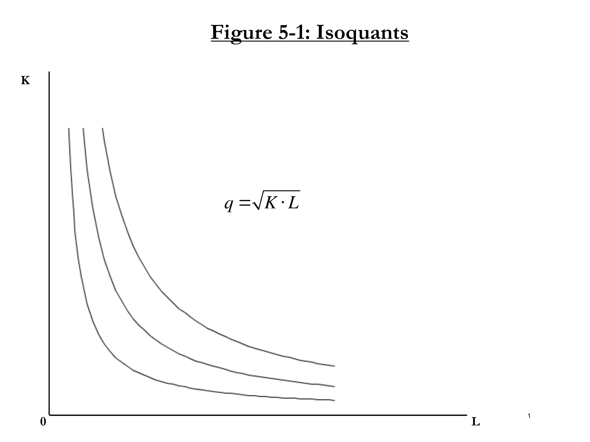
Figure 5-1: Isoquants for q = √(K·L). Each curve represents a different output level.
6.4 Isoquant Map (Graphical Representation)
Picture: Graph with K on vertical axis, L on horizontal axis
- Each curve represents a different output level (q = 1, q = 2, q = 3, ...)
- Curves further from origin = higher output
- Along each curve, output is constant
For q = √(L×K), the isoquant for q = 4:
4 = √(L×K) → 16 = L×K → K = 16/L
This is a rectangular hyperbola.
6.5 Properties of Isoquants (Same as Indifference Curves!)
| Property | Meaning | Why? |
|---|---|---|
| 1. Further out is better | Higher isoquants = more output | More inputs → more output |
| 2. Slope downward | Trade-off between L and K | To keep q constant, ↑L requires ↓K |
| 3. Don't cross | Same logic as indifference curves | If they crossed, same inputs would give different outputs |
| 4. Convex to origin | Diminishing MRTS | Diminishing marginal products |
6.6 What Determines the Shape of Isoquants?
Student Answer: "Depending on how the different inputs go with each other?"
Gruber: "Exactly. It's going to depend on the substitutability of the different inputs. The more substitutable, the straighter is the isoquant; the less substitutable, the more bent is the isoquant."
6.7 Extreme Cases
| Case | Production Function | Isoquant Shape | Example |
|---|---|---|---|
| Perfect Substitutes | q = L + K | Straight lines (slope = -1) |
"Harvard graduates and Beanie Babies" 😄 (Gruber's joke about perfect substitutability) |
| Normal Case | q = √(L×K) | Smooth curves (convex) |
Most production processes |
| Perfect Complements | q = min(L, K) | L-shaped (right angles) |
"Cereal and cereal boxes" "For every amount of cereal, you need a box" |
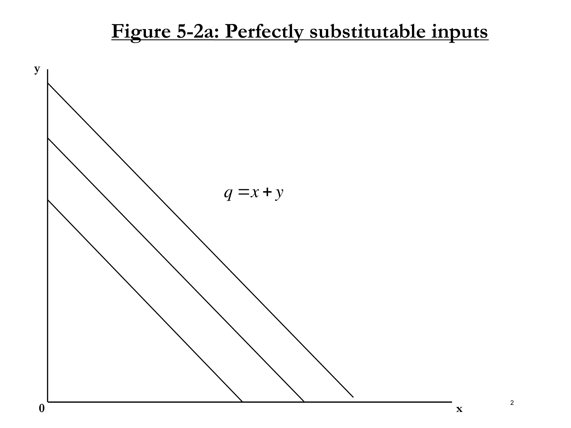
Figure 5-2a: Perfect Substitutes (q = x + y)
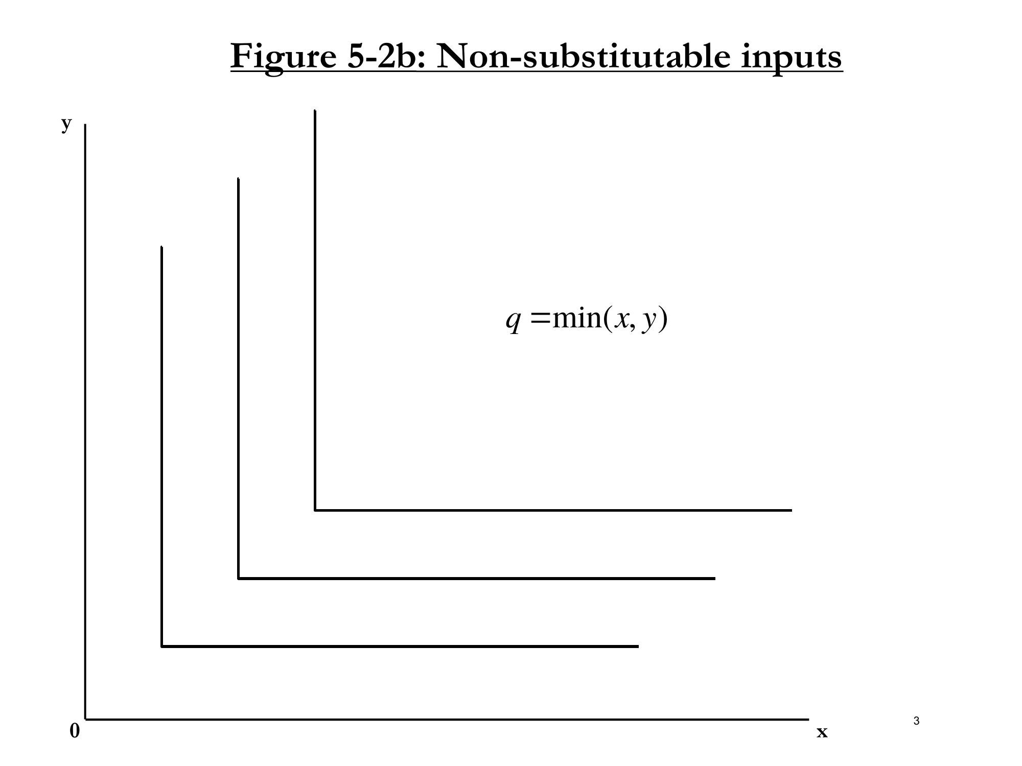
Figure 5-2b: Perfect Complements (q = min(x, y))
Cereal Box Example (Perfect Complements):
"For every amount of cereal you got, you got to have a box. If you only have one box, it doesn't matter how much cereal you have, it's just going to sit there."
"Just like the indifference curves for left shoe, right shoe—this is cereal, cereal boxes, things which are non-substitutable."
Reality: "Nothing's ever at the extremes. We'll generally be in between these two cases."
7. Marginal Rate of Technical Substitution (MRTS)
Terminology Warning: "Now with consumers, you had marginal rate of substitution and marginal rate of transformation, MRS and MRT. Now I'm going to have MRTS, which is the marginal rate of technical substitution—just to really mess you up."
7.1 Definition
MRTS: The rate at which you can trade off labor and capital while producing the same quantity of output.
MRTS = dK/dL|q constant = Slope of isoquant
7.2 Mathematical Derivation
Question: What happens with a marginal increase in L and marginal decrease in K, staying on the same isoquant?
Step 1: Along an isoquant, output is constant (dq = 0)
Step 2: Total differential of production function:
dq = (∂q/∂L)dL + (∂q/∂K)dK = MPL·dL + MPK·dK
Step 3: Set dq = 0 (staying on isoquant):
0 = MPL·dL + MPK·dK
Step 4: Solve for dK/dL:
MPK·dK = -MPL·dL
dK/dL = -MPL/MPK = MRTS
Compare to Consumer Theory:
| MRS (Consumer) | = -MUx/MUy | Slope of indifference curve |
| MRTS (Producer) | = -MPL/MPK | Slope of isoquant |
7.3 Example Calculation
For q = √(L × K) = L0.5K0.5:
Step 1: Find MPL
MPL = ∂q/∂L = 0.5 × L-0.5 × K0.5 = 0.5 × K/√(LK) = 0.5 × √(K/L)
Step 2: Find MPK
MPK = ∂q/∂K = 0.5 × L0.5 × K-0.5 = 0.5 × L/√(LK) = 0.5 × √(L/K)
Step 3: Calculate MRTS
MRTS = -MPL/MPK = -[0.5√(K/L)] / [0.5√(L/K)]
MRTS = -K/L
"For this production function, that's the marginal rate of technical substitution."
7.4 Interpreting MRTS Along an Isoquant
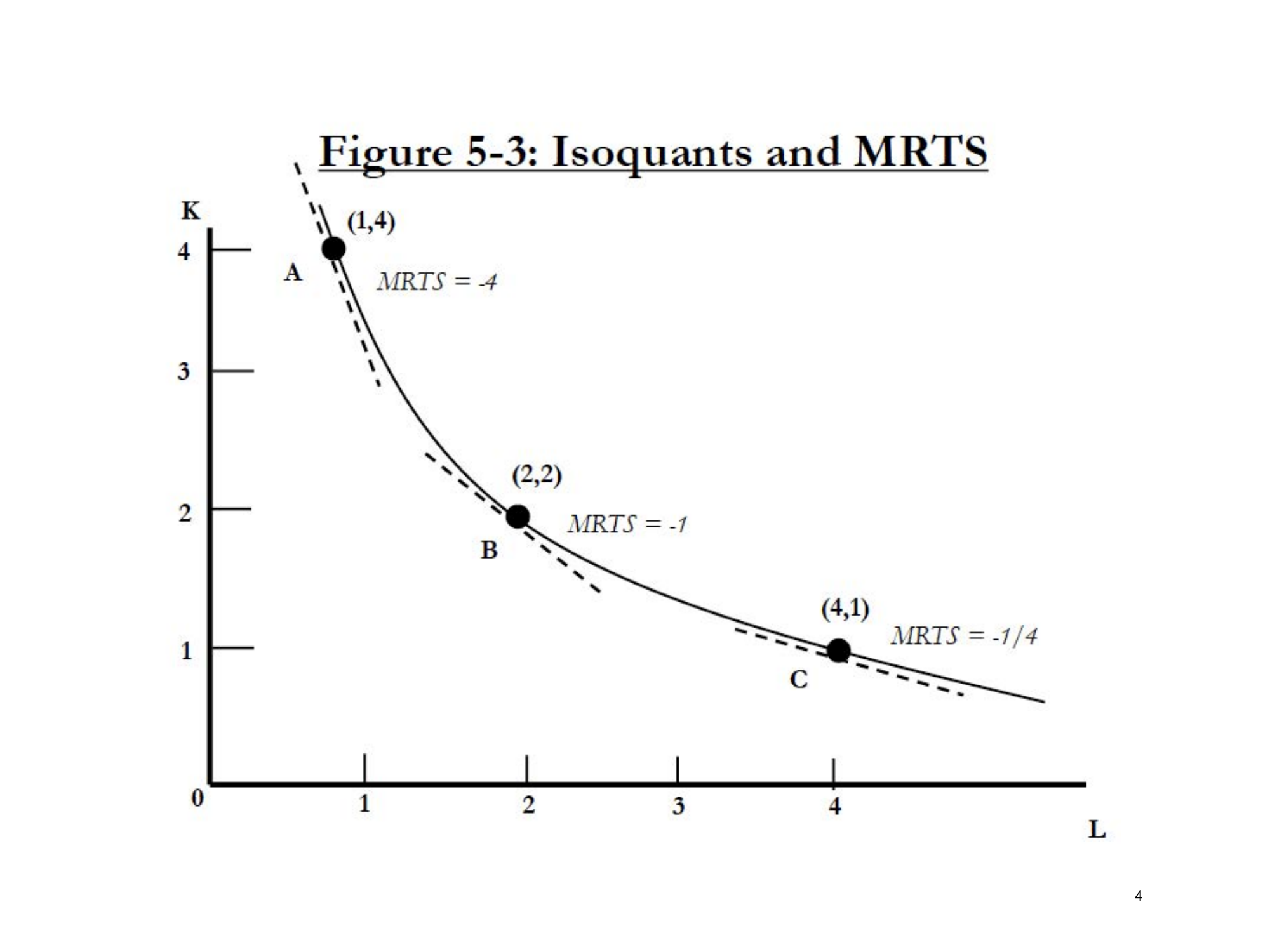
Figure 5-3: Isoquants and MRTS. Points A(1,4), B(2,2), C(4,1) show how MRTS changes along the isoquant.
| Point | Situation | K/L | MRTS | Interpretation |
|---|---|---|---|---|
| Point A (Upper left) |
Little L, lots of K e.g., 1 worker, 4 shovels |
4/1 = 4 | -4 | Willing to give up 4 units of K for 1 more L |
| Point B (Middle) |
Equal L and K e.g., 2 workers, 2 shovels |
2/2 = 1 | -1 | Willing to trade 1:1 |
| Point C (Lower right) |
Lots of L, little K e.g., 4 workers, 1 shovel |
1/4 = 0.25 | -1/4 | Willing to give up only 1/4 K for 1 more L |
Intuition:
"When you've got four shovels and one worker, you'd happily give up shovels to get more workers. So you want to move to the right."
"Likewise, at point C, you've got four workers and one shovel. That's doing you no good. You'd happily give up a worker to get a shovel, so you want to move to the left."
Why? Because marginal products are diminishing! When you have lots of something, its marginal product is low, so you're willing to trade it away.
7.5 Diminishing MRTS
As you move along an isoquant from upper-left to lower-right:
- L increases, K decreases
- MPL decreases (diminishing returns to L)
- MPK increases (less K means higher marginal product)
- |MRTS| = MPL/MPK decreases
This is why isoquants are convex to the origin!
8. Returns to Scale
Note: "I'm going to talk about two things which are not parallel to consumer theory."
"Producer theory is one step harder than consumer theory. It's all the fun stuff for consumer theory plus one additional step."
8.1 The Question
Returns to Scale: What happens when we increase all inputs proportionally?
"When you say in your mind, 'what happens when a firm gets bigger?', you're thinking, what happens when everything increases? When all inputs increase proportionally is our notion of how a firm gets bigger."
8.2 Formal Definition
Consider multiplying all inputs by a factor t > 1:
f(tL, tK) compared to t × f(L, K)
8.3 Three Types of Returns to Scale
| Type | Condition | Meaning | Example |
|---|---|---|---|
| Constant Returns (CRS) | f(2L, 2K) = 2f(L,K) | Double inputs → Double output | "Sort of a natural intuition" |
| Decreasing Returns (DRS) | f(2L, 2K) < 2f(L,K) | Double inputs → Less than 2× output | Crowding, coordination problems |
| Increasing Returns (IRS) | f(2L, 2K) > 2f(L,K) | Double inputs → More than 2× output | Specialization benefits |
8.4 Example: q = √(L × K)
Let's check: f(2L, 2K) = √(2L × 2K) = √(4LK) = 2√(LK) = 2f(L, K)
Result: This production function exhibits constant returns to scale!
8.5 Why Decreasing Returns?
"Think about the idea that basically, if you're still trying to dig a hole, there's one guy with one shovel, you go two guys with two shovels, they're in each other's way, they can't quite work as efficiently as one guy with one shovel because you're still trying to dig one hole."
Causes of DRS:
- Coordination problems
- Communication difficulties
- Workers getting in each other's way
- Management challenges
8.6 Why Increasing Returns?
"That might arise through something like the fact that when the firm gets bigger, it can specialize more. So maybe as a firm gets bigger and bigger, it can get better and better at what it does, and production can become more and more efficient."
Causes of IRS:
- Specialization and division of labor
- Bulk purchasing discounts
- Fixed costs spread over more output
- Network effects
8.7 Why This Matters: The One-Firm Economy
"This is an important concept because basically, this is how we think about economies growing. This is the core of any model of economic growth."
Key Insight:
"Typically, economists do not believe that there is everywhere and always increasing returns to scale. We typically believe returns to scale may increase initially as you specialize as a firm, but eventually you have to decrease."
The Crucial Question:
"And the reason we believe that, or at least believed that, was that if there was always and forever increasing returns to scale, how many firms would there be in the economy?"
ONE.
"Because it could always just do better by getting bigger and bigger and bigger."
8.8 Modern Complication: Tech Giants
"Now it turns out, for search engines, maybe that's not such a bad description. We'll see in the trial that's going on now where Google may get broken up."
"So it may be that increasing returns to scale may last longer than we thought as economists."
The pattern economists expect:
- Initially: Increasing returns (specialization benefits)
- Eventually: Decreasing returns (coordination problems dominate)
"But typically, we think of firms as maybe initially having increasing returns to scale, and then eventually as they mature, having decreasing returns to scale."
8.9 Returns to Scale vs Diminishing Marginal Product
Important Distinction:
| Diminishing MP | Returns to Scale | |
|---|---|---|
| What changes? | ONE input (others fixed) | ALL inputs (proportionally) |
| Time frame | Short-run | Long-run |
| Can coexist? | Yes! A function can have diminishing MP but constant or increasing returns to scale | |
9. Productivity: The Missing Piece
"One of the most exciting topics in economics is thinking about productivity. One of the most famous—and the idea of productivity comes actually from a very famous application from 1798 of the idea of decreasing returns to scale or diminishing marginal product."
9.1 The Malthusian Prediction (1798)
Thomas Malthus's Argument:
- "Think about the production of agriculture. There's essentially two inputs: people and land."
- "The difference between capital and land is land is always fixed. Even in the long-run. There's only so much land. We got the Earth. Unless we go colonize another planet."
- "There's a fixed amount of land, so that means that the marginal product of labor must be everywhere diminishing."
- "That means that eventually, we're going to starve."
9.2 Malthus's Grim Vision
"Malthus actually said that there would be cycles—the world would be marked by cycles of starvation."
The Malthusian Cycle:
- Population grows
- Unable to produce enough food (diminishing MPL)
- Many people die from starvation
- Population falls to sustainable level
- Food production adequate → population grows again
- Return to step 1...
"Really not a very happy picture of the future."
(Gruber describes Malthus as "a very, I think, probably pretty depressed philosopher")
9.3 What Actually Happened
Since Malthus wrote that book in 1798:
| World Population | Increased roughly 1,000% (about 100×) |
| Starvation | "And we are fatter than ever." |
| Food per capita | "World food consumption per capita is actually up since 1950 despite the fact that world population has grown." |
9.4 Important Caveat: Famines Still Exist
"Not that there's not starvation. And let's be clear, there's horrible starvation around the world."
Amartya Sen's Nobel Prize-winning observation:
"There's never been a famine in a democracy."
"So we think about famines and starvation all over the world, remember, that's a political failure, not technological failure. There's never been a famine in a democracy. Famines only happen when corrupt governments don't spread the food they need to the people who need to get it."
9.5 What Did Malthus Miss?
Technology! Productivity!
q = A × f(L, K)
where A = Productivity factor (Total Factor Productivity)
"He was right that the amount of land is fixed, but he missed the fact that the way we use that land will get more and more productive over time. He missed all the technology that was going to come. He missed the productivity improvements that we were going to see."
9.6 Examples of Productivity Improvements
| Industry | Innovation | Impact |
|---|---|---|
| Agriculture |
• Fertilizers • Farm machinery • Disease-resistant seeds • Better land management |
Much more food from same land |
| Cars (Henry Ford) | "Assembly line where basically, you had interchangeable parts, and you had a conveyor belt where people could just specialize in screwing this bolt in over and over again, and they could do it much faster." | "Cut the cost of car production in half almost overnight" |
| Cars (Tata Nano) | "Much lighter than other cars. Much smaller, but they do things like putting the wheels way out on the edge instead of under the car to create more room for people to sit in. And they minimize the parts." | $2,500 car! |
| Cars (Tesla) | Electrification of the automobile fleet | "One of the most major innovations in our automobile industry in decades... despite what we think about Elon Musk, it's a pretty cool car." |
10. Productivity and Standard of Living
10.1 What Determines Standard of Living?
Standard of Living = How much stuff we get to consume per person
Standard of Living ∝ q/Population = A × f(L, K)/Population
10.2 Three Ways to Increase Standard of Living
| Factor | What It Means | Cost |
|---|---|---|
| 1. Labor (L) | Work harder/longer | "Working harder is costly. You've got to work harder, it sucks." |
| 2. Capital (K) | Build more machines | "You got to build a machine, you need to use stuff to build a machine." |
| 3. Productivity (A) | Be more efficient | "Boom, you got more. A brilliant idea, and suddenly, boom, you got more stuff for everyone." |
"What's great about productivity is these two are expensive. Working harder is costly. Capital, you got to build a machine. Productivity, boom, you got more. A brilliant idea, and suddenly, boom, you got more stuff for everyone."
"So productivity is the magic that makes economic growth happen almost costlessly."
"And as a result, productivity is the central determinant of our standard of living."
10.3 US Productivity Growth Over Time
| Period | Growth Rate | What It Meant |
|---|---|---|
| WWII - 1973 | ~2.5%/year | "Working just as hard with just as many machines, we could each consume 2.5% more stuff every single year just magically through the growth in productivity." |
| 1973 - mid-1990s | < 1%/year | "If we wanted more stuff, we had to work harder, get more machines." |
| Mid-1990s - Mid-2000s | ~2.3%/year | "We thought, aha! The IT revolution is here." |
| After 2005 | ~1%/year | "It stopped and productivity is back down again... we're not really growing, we're not really innovating." |
10.4 The IT Paradox
"The IT revolution started in the late '80s, but productivity didn't increase. People were saying, well, where's the IT revolution?"
Famous Quote (Robert Solow):
"You can see the computer age everywhere but in the productivity statistics."
"You guys have no idea how different life is now than it was 25 years ago in terms of the internet and everything you have, but somehow, we're not that much more productive as an economy."
11. Four Key Questions About Productivity
Question 1: Why No Long-Lasting IT Effects?
"Why did the IT revolution cause this brief burst and then eventually kind of wear off?"
"Is it because basically all our innovation is watching TikTok and not in making stuff? I don't know."
The puzzle: Life is radically different from 25 years ago, but we're not that much more economically productive. Why not?
Possible explanations:
- Measurement problems (we're not capturing value correctly)
- Innovation is in consumption, not production
- Benefits going to leisure, not measured output
- Takes time for technology to diffuse
Question 2: Where Does Productivity Come From?
"I said it was free, it's not free, it's not magical. Productivity is through real things."
| Source | How It Works | Who Does It |
|---|---|---|
| Education | "As we educate people to make them smarter, make them more creative, they'll think of cool new ideas." | Schools, universities |
| Firm R&D | "As firms do research and development... they think up new ideas. And they develop new products." | Private companies |
| Public R&D | "Like the National Science Foundation... The National Institutes of Health fund a lot of research." | Government (NSF, NIH) |
Key Distinction:
- Firms: Do "applied research" - take basic ideas and turn them into products
- Government: Funds the "basic research" that underlies those products
"So basically, there are things we can do as a society to increase our productivity—we don't just sit back and let it happen. Having more educated population, more investments in R&D. Those can really make a difference in terms of how fast we grow."
Question 3: How Should We Spend Productivity?
"Imagine you have a cool new idea that can make things more efficient. Take Henry Ford's idea. He could do two things with that:"
| Option 1: More q | Make more cars (more stuff) |
| Option 2: Less L | Give people more time off (more leisure) |
"If A goes up, you can reduce L, and with the same amount of output. There's no reason an increase in A has to go into more q. An increase in A could go into less L, which people like. They like time off."
The Hardest Thing About Teaching at MIT
"One thing we learn in this class, the hardest thing about teaching a class at MIT, the single hardest thing is in the real world, people actually don't like work. I find this hard to believe, guys, but in the real world, people would rather not be at work than at work."
US vs Europe: Different Choices
| United States | Europe | |
|---|---|---|
| Starting vacation | 2 weeks | 6 weeks |
| Working years | Age 20 to 65 | Age 25 to 60 |
| Hours per week | More | Less |
| Productivity goes to: | More stuff | More leisure |
"What's the better thing to have? Good question. When I was young, I probably thought stuff. Now that I'm older, I might think time off."
The Pandemic Effect
"The pandemic may have shook this up in the US. The pandemic was the first chance that people had to actually be at home and say, wait a second, maybe I don't want to work that hard."
Post-pandemic changes:
- Huge reduction in labor supply
- Many people retired early
- People aren't working as hard
- People want better jobs
- People want to work from home
"So the pandemic really shook things up in terms of people maybe starting to value their leisure more than maybe they did before."
Question 4: Who Gets A? (The Distribution Question)
"Which group in society benefits from a more productive economy?"
| Period | Who Benefited? |
|---|---|
| WWII - 1973 | "Pretty much every group in society saw that increase. The poorest people saw their incomes go up about 2.5% a year, the richest people saw their incomes go up to about 2.5% a year." |
| Since mid-1970s | "Virtually all of the benefit of increased productivity has gone to the richest members of society, the people that own the capital, and not to the workers." |
The Numbers
| Average worker's purchasing power | "Not much higher than what you could buy with that wage in 1980." |
| Top 1% share of income | 26% (1989) → 35% (today) |
| 2021 (post-pandemic recovery) | "The top 1% of earners saw their incomes increase by 9% while everyone else saw their incomes decrease." |
The Bottom Line:
"A doesn't magically go to everyone. It's not like a more productive economy, everyone benefits. That's determined by a set of decisions made by individual actors in the economy and by the government. And that's what we'll talk about later in the semester, is how does the government think about those decisions?"
"And that comes to the topic of economic fairness, which we won't spend nearly enough time on, but we will come back to towards the end of the semester."
Key Takeaways
| # | Concept | Key Point |
|---|---|---|
| 1 | Firm's Goal | Maximize profits = Minimize costs (since demand & competition largely given) |
| 2 | Production Function | q = f(L, K) — the "black box" that converts inputs to outputs |
| 3 | Factors of Production | Labor (L, wage w) and Capital (K, rental rate r) — "both things you rent" |
| 4 | Short vs Long Run | Short: K fixed, L variable. Long: both variable. "Days vs decades" |
| 5 | Diminishing MP | Each additional worker adds value, but less and less (hole-digging example) |
| 6 | Isoquants & MRTS | Parallel to indifference curves & MRS; MRTS = -MPL/MPK |
| 7 | Returns to Scale | What happens when firm scales ALL inputs — constant, increasing, or decreasing |
| 8 | Productivity (A) | The "magic" of economic growth — almost free! But who benefits? |
Producer Theory ↔ Consumer Theory Parallels
| Consumer Theory | Producer Theory |
|---|---|
| Utility Function U(x,y) | Production Function f(L,K) |
| Indifference Curves | Isoquants |
| MRS = MUx/MUy | MRTS = MPL/MPK |
| Diminishing Marginal Utility | Diminishing Marginal Product |
| Maximize Utility | Maximize Profits (= Minimize Costs) |
| Budget Constraint: Pxx + Pyy = I | Isocost Line: wL + rK = C (coming in future lectures) |
Key Terms Glossary
| Term | Definition |
|---|---|
| Production Function | q = f(L, K); Mathematical relationship showing what output is technically feasible given inputs |
| Labor (L) | Hours of work; price = wage (w) |
| Capital (K) | Machines, buildings, land; price = rental rate (r) |
| Short-Run | Period where some inputs are fixed (typically K) |
| Long-Run | Period where all inputs are variable |
| Marginal Product (MP) | Additional output from one more unit of input: MPL = ∂q/∂L |
| Diminishing MP | ∂²q/∂L² < 0; each additional worker adds less and less (but still positive!) |
| Isoquant | Combinations of L and K producing the same output; like indifference curve for producers |
| MRTS | Marginal Rate of Technical Substitution = -MPL/MPK; slope of isoquant |
| Returns to Scale | What happens when ALL inputs scale proportionally (constant, increasing, or decreasing) |
| Productivity (A) | Technology factor that makes inputs more efficient; q = A × f(L,K) |
Last updated: 2025-01-11