MIT 14.01 Principles of Microeconomics | Fall 2023 | Prof. Jonathan Gruber
Lecture 4: Demand Curves and Income/Substitution Effects
한국어Core Message
"The last two lectures we started building that basis. And today we'll show you where demand curves actually come from."
Demand curves are derived by finding optimal consumption at different prices. When prices change, two effects occur simultaneously: the substitution effect and the income effect.
Consumer Theory Progress
| Step 1 (Lec 2) | Preferences → Utility Function → Indifference Curves | ✓ Done |
| Step 2 (Lec 3) | Budget Constraint → Constrained Choice | ✓ Done |
| Step 3 (Lec 4) | Derive Demand Curves | ← Today |
1. Deriving a Demand Curve
Definition
Demand Curve: The relationship between the price charged for a good and the consumer's desired quantity of the good.
Setup (Review)
| Utility Function | U = √(S × C) |
| Budget Constraint | Y = PS × S + PC × C |
| Income (Y) | $24 |
| Price of Pizza (PS) | $4 |
| Price of Cookies (PC) | $2 (initial) |
Step 1: Solve for Optimal Consumption
Optimization Condition: MRS = MRT
-S/C = -PC/PS = -2/4 = -1/2
→ S = C/2 ... (Equation 1)
Budget Constraint:
24 = 4S + 2C
Substitute (1): 24 = 4(C/2) + 2C = 4C
→ C* = 6, S* = 3
Step 2: Change Price of Cookies
| PC | MRT | Optimization | Result | Point |
|---|---|---|---|---|
| $4/3 | -1/3 | S = C/3 | C=9, S=3 | C |
| $2 | -1/2 | S = C/2 | C=6, S=3 | A |
| $3 | -3/4 | S = 3C/4 | C=4, S=3 | B |
Step 3: Draw the Demand Curve
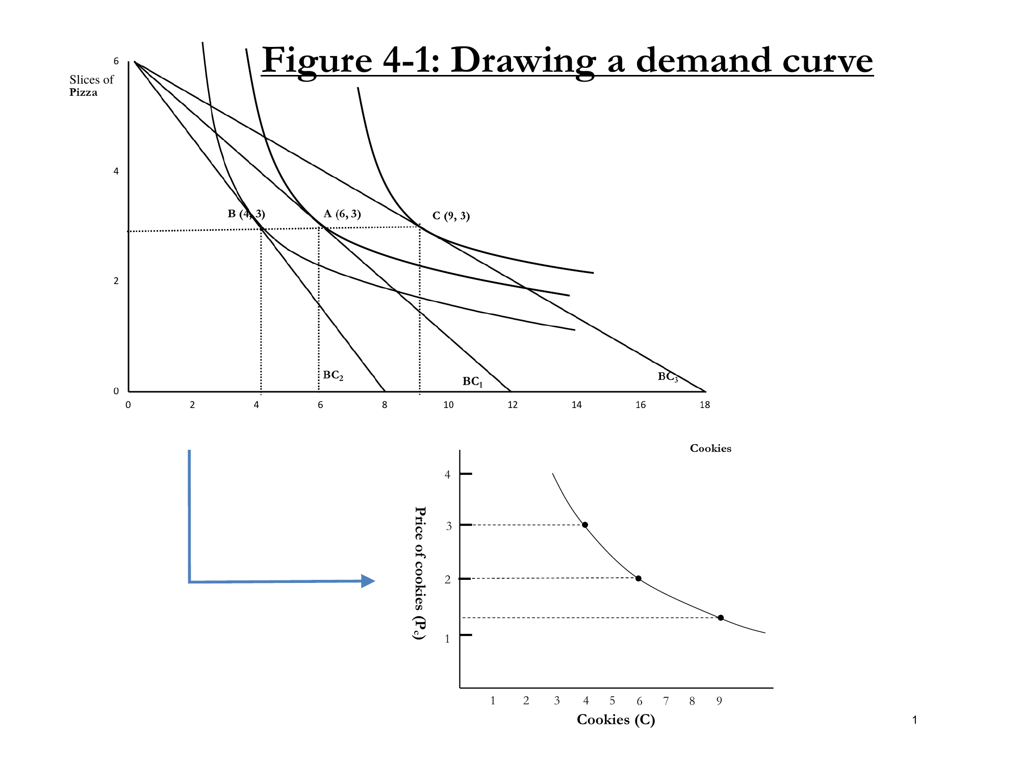
Figure 4-1: Deriving the Demand Curve from Utility Maximization
Key Insight: The demand curve is derived by optimizing utility at different prices and finding which quantity you want at each price.
Student Question: "Why doesn't pizza quantity change?"
"Great point. Someone noticed. That as we varied the price of cookies, the number of slices of pizza did not change. That is not a general law. That is a specific feature of this utility function."
This is called a flat cross-price consumption curve — a special property of this particular utility function that makes calculations simpler.
2. Elasticity of Demand
Definition
ε = (ΔQ/Q) / (ΔP/P) ≈ (dQ/dP) × (P/Q)
"How responsive is demand to price changes?"
Extreme Cases
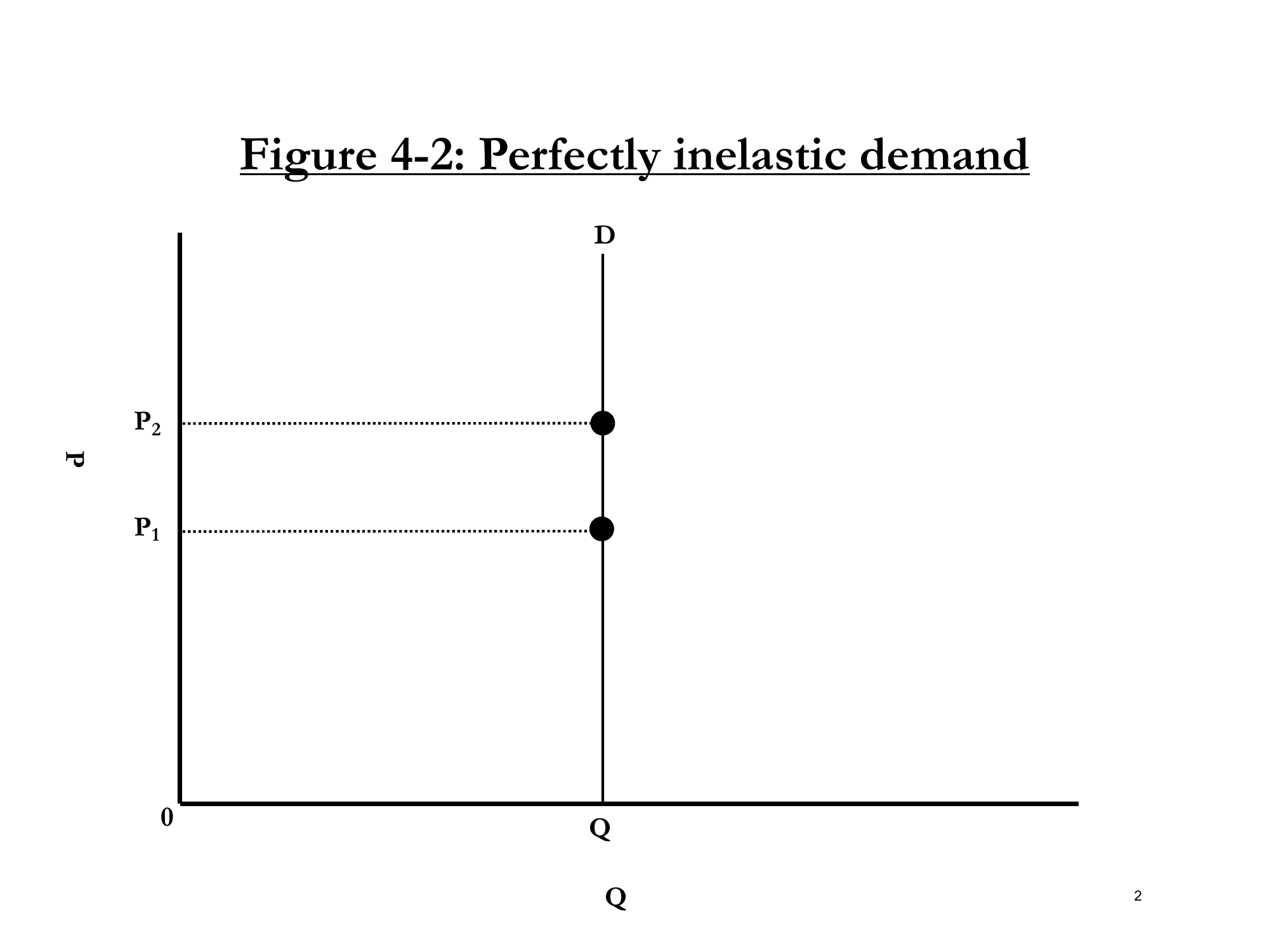
Figure 4-2: Perfectly Inelastic (ε = 0)
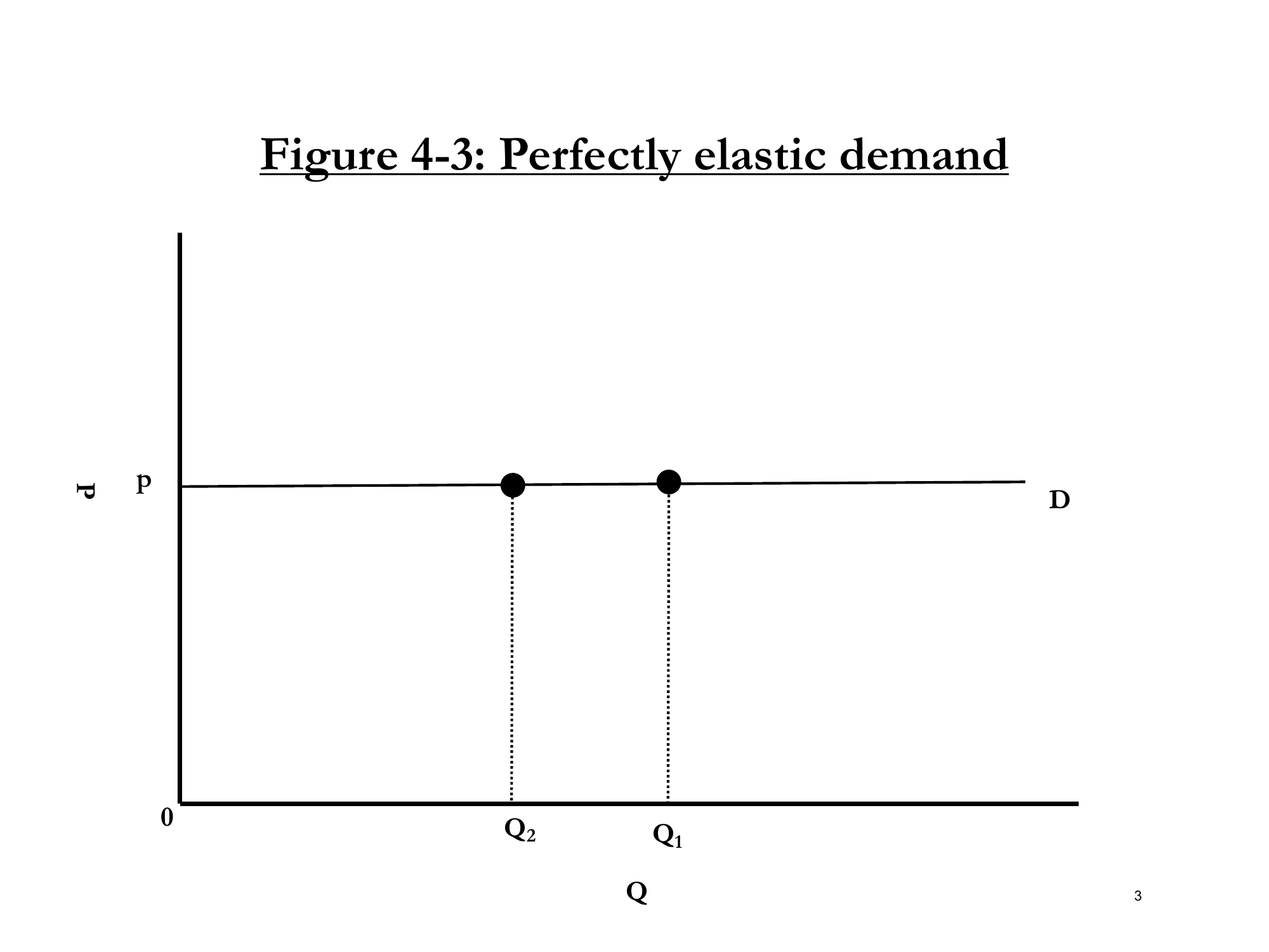
Figure 4-3: Perfectly Elastic (ε = -∞)
| Type | ε Value | Curve Shape | Substitutes | Example |
|---|---|---|---|---|
| Perfectly Inelastic | ε = 0 | Vertical | None | Insulin |
| Inelastic | -1 < ε < 0 | Steep | Few | Gas, Water |
| Elastic | ε < -1 | Flat | Many | Luxury goods |
| Perfectly Elastic | ε = -∞ | Horizontal | Infinite | McDonald's vs Burger King |
Key Principle: Substitutability = Elasticity
"Here's the key feature that differentiates elasticity. It's substitutability. Goods with no substitutes are not elastic. Goods with lots of substitutes are very elastic."
Classroom Examples
Student: "Gas?"
Gruber: "Gas would be somewhat inelastic because you got to get to work. On the other hand, there's a bus, there's your bike. You could walk, you could buy a new car. So it's not perfectly inelastic."
Student: "Insulin?"
Gruber: "Insulin is the classic example we use. There's no substitute. When you're having diabetic trauma for insulin, you will not say, 'it's $1 more, I'm just going to die.'"
3. Income and Demand: Engel Curves
What Happens When Income Changes?
| Income (Y) | Cookies (C*) | Pizza (S*) | Point |
|---|---|---|---|
| $16 | 4 | 2 | C |
| $24 | 6 | 3 | A |
| $32 | 8 | 4 | B |
Key: Price ratio unchanged → MRS = MRT condition unchanged
Budget line shifts parallel (not pivots)
The Engel Curve
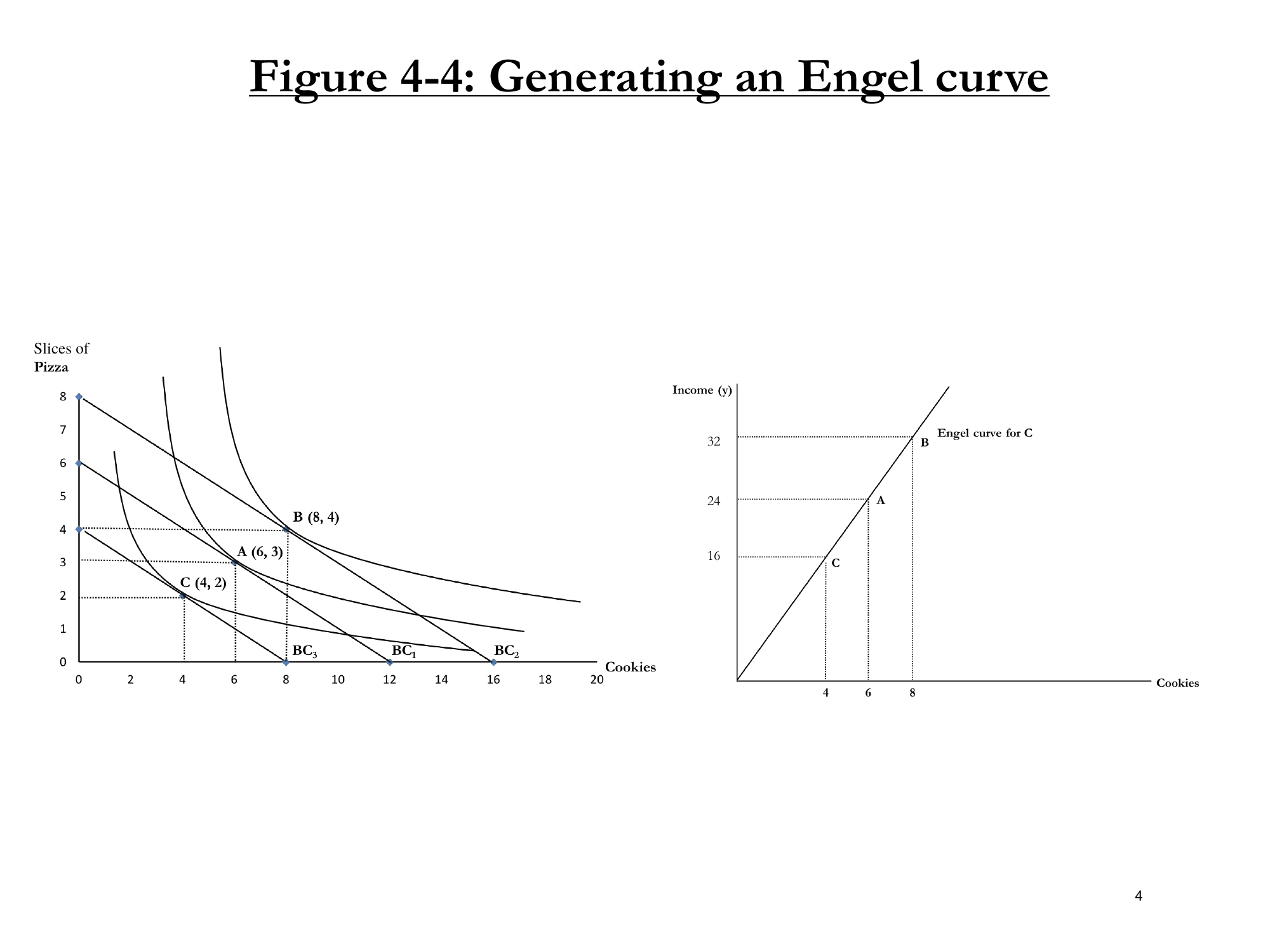
Figure 4-4: Generating an Engel Curve
Definition: The relationship between income and quantity demanded
γ = (ΔQ/Q) / (ΔY/Y) ≈ (dQ/dY) × (Y/Q)
Income Elasticity of Demand
Gamma (γ) vs Epsilon (ε)
"Gamma is much more interesting than epsilon. Epsilon, some negative number, 0 to minus infinity. Gamma can have a much larger range."
| Elasticity | Range | Constraint |
|---|---|---|
| ε (Price) | 0 to -∞ | Always ≤ 0 |
| γ (Income) | -∞ to +∞ | No constraint |
4. Classification of Goods by Income Elasticity
Complete Classification
| Type | γ Value | Meaning | Example |
|---|---|---|---|
| Inferior | γ < 0 | Income↑ → Demand↓ | Ramen |
| Necessity | 0 < γ < 1 | Income↑ → Budget share↓ | Rent, Basic food |
| Luxury | γ > 1 | Income↑ → Budget share↑ | Restaurant meals, Watches |
Ramen: The Ultimate Inferior Good
"Ramen is the example. Ramen is the ultimate inferior good. No one wants to eat ramen. I realize there's fancy ramen restaurants, but nobody should go there."
"People eat ramen because it's cheap. As you get richer, you consume less ramen."
Necessity vs Inferior: Key Distinction
| Inferior | Income↑ → Absolute quantity decreases |
| Necessity | Income↑ → Quantity increases, but slower than income |
"Rent is the perfect example. Richer people have nicer apartments than poorer people, but richer people spend a smaller share of their budget on apartments than do poorer people."
5. Mechanics of a Price Change
Why This Matters
"When a price changes, two things happen simultaneously. You may not realize it, but actually when a price changes, two things happen."
Two Simultaneous Effects
| Effect | Definition | Mechanism |
|---|---|---|
| Substitution Effect | Shift away from relatively expensive good | Relative prices change |
| Income Effect | You're effectively richer or poorer | Real purchasing power changes |
"When a price changes, two things happen. Goods become differentially attractive and you're richer or poorer. And both things drive your response to that price change."
6. Decomposing Income and Substitution Effects
Example Setup
- Starting Point (A): C = 6, S = 3 (on BC1)
- Price Change: PC: $2 → $3
- Ending Point (C): C = 4, S = 3 (on BC2)
Measuring the Substitution Effect
Definition: Change in quantity holding utility constant
ΔQ|Ū
Graphical Method: Draw an imaginary budget constraint BC' with two features:
- Parallel to new budget constraint (reflects new price ratio -3/4)
- Tangent to original indifference curve (keeps utility constant)
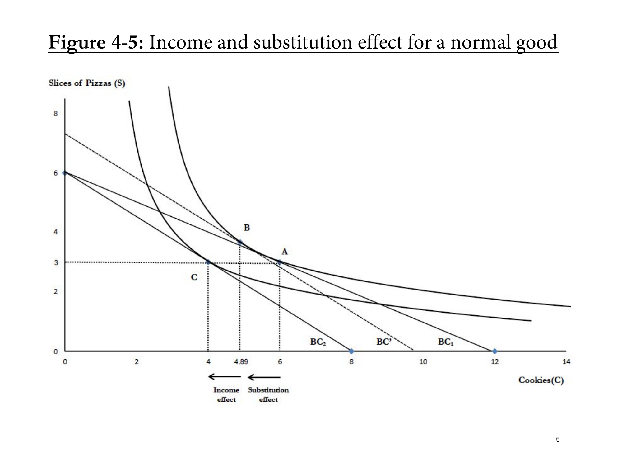
Figure 4-5: Income and Substitution Effects for a Normal Good
"We're showing you the change in quantity you get at a constant utility. How do we keep utility constant? We stay on the same indifference curve."
Results
| Movement | Effect | Cookies |
|---|---|---|
| A → B | Substitution Effect | 6 → 4.89 |
| B → C | Income Effect | 4.89 → 4 |
| A → C | Total Effect | 6 → 4 |
Substitution Effect is Always Negative
Mathematical Proof:
- At tangency: MUC/MUS = PC/PS
- PC/PS went up (cookies more expensive)
- MUC/MUS must go up to maintain equality
- To raise MUC → consume fewer cookies (diminishing MU!)
- To lower MUS → consume more pizza
Conclusion: Price↑ → Substitution effect is always negative
Income Effect Sign Depends on Good Type
Why are you "effectively poorer"?
"Your income itself hasn't fallen, but your resources have, what you can buy with that income has fallen. You're effectively poor."
Student: "Your opportunity set has been constricted."
Gruber: "Your opportunity set has been constricted."
| Good Type | When Income↓ | Income Effect |
|---|---|---|
| Normal | Demand↓ | Negative (same as substitution) |
| Inferior | Demand↑ | Positive (opposite to substitution) |
7. Inferior Good Example: Steak vs Potatoes
Setup
"Figure 4.6 is no longer pizza and cookies. Figure 4.6 is now steak and potatoes. Because pizza and cookies are both normal goods."
"Potatoes is the classic inferior good. Poor people, especially back in the day, used to have to eat potatoes because they were cheap to grow and very filling."
| Income | $25 |
| Price of Steak | $5 |
| Price of Potatoes | $1 → $3 |
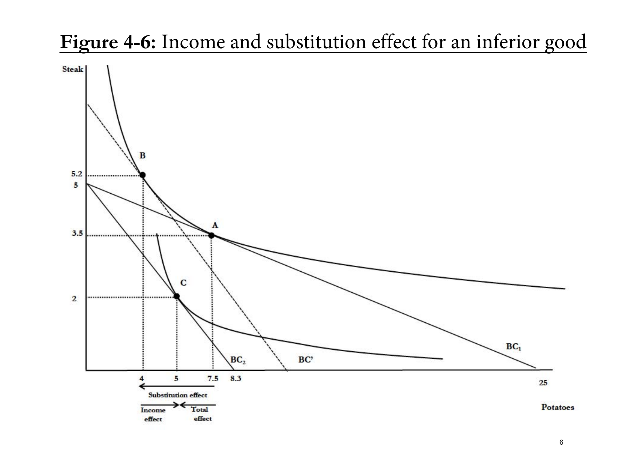
Figure 4-6: Income and Substitution Effects for an Inferior Good (Potatoes)
Decomposition
| Effect | Potatoes | Explanation |
|---|---|---|
| Substitution (A→B) | 7.5 → 4 ↓ | Price↑ → want less (always!) |
| Income (B→C) | 4 → 5 ↑ | Poorer + Inferior good → want more! |
| Net Effect | 7.5 → 5 ↓ | Effects work against each other |
"The income effect goes the other way because potatoes are an inferior good. In other words, now that you're so poor, now potatoes are so expensive, you don't have enough money for steak anymore. So you got to have more potatoes. It's ironic, right?"
8. Giffen Goods
Definition
A Giffen good is an inferior good where the income effect dominates the substitution effect, resulting in an upward-sloping demand curve.
Price↑ → Demand↑ (violates law of demand!)
Do They Exist?
"I like the name Giffen because it rhymes with Griffin. And Griffins are imaginary. Giffen goods are also largely imaginary. It's a great theoretical concept, but they don't really exist."
The Irish Potato Famine Story
Claim: During the potato blight, potato prices rose but per capita potato consumption rose. Therefore, potatoes are a Giffen good!
Gruber's Rebuttal:
"Here's what they got wrong. Here's where empirical economics is fun. They miss the fact that what other effect did the potato blight have? It chased all the people who could afford it out of Ireland. The only people who were left were super poor."
"So yeah, on average, potatoes per person went up. It's a Giffen good. What you're missing is the capitas are different. Each person needs more potatoes. It's just the non-potato eaters left."
Giffen vs Veblen Goods
Student: "A Veblen good?"
Gruber: "A Veblen good is a totally different concept. That's the concept that basically you want more when the price is up because you care about your social standing. But that's a behavioral economics thing. We'll come back to that type of behavior. It's not a standard economics effect."
9. Complete Summary Chart
Normal Goods
| Price Change | Substitution | Income | Net |
|---|---|---|---|
| ↑ | − | − | − (Clear) |
| ↓ | + | + | + (Clear) |
Inferior Goods
| Price Change | Substitution | Income | Net |
|---|---|---|---|
| ↑ | − | + | ? (Unclear) |
| ↓ | + | − | ? (Unclear) |
Why This Matters
"I'll tell you why we care in about six lectures. Because it turns out when you make your decisions about how hard you're going to work or how much you're going to save, income substitution effects are going to start to work against each other."
Key Takeaways
| # | Concept | Key Point |
|---|---|---|
| 1 | Demand Curve Derivation | Calculate optimal quantity at various prices |
| 2 | Elasticity | More substitutes = More elastic |
| 3 | Engel Curve | Income-demand relationship; γ classifies goods |
| 4 | Substitution Effect | Always opposite sign of price change |
| 5 | Income Effect | Same direction for normal; opposite for inferior |
| 6 | Giffen Goods | Theoretical only; don't exist in practice |
Key Terms
| Term | Definition |
|---|---|
| Demand Curve | Relationship between price and quantity demanded |
| Price Elasticity (ε) | Responsiveness of demand to price changes |
| Engel Curve | Relationship between income and quantity demanded |
| Income Elasticity (γ) | Responsiveness of demand to income changes |
| Normal Good | γ > 0; demand increases with income |
| Inferior Good | γ < 0; demand decreases with income |
| Substitution Effect | Demand change due to relative price change (utility constant) |
| Income Effect | Demand change due to change in real purchasing power |
| Giffen Good | Inferior good where income effect > substitution effect |
Last updated: 2025-01-10